Model Definition
For the modeling and optimization of an energy system, parameters for all system components must be given in the model generator using the enclosed .xlsx file (editable with Excel, LibreOffice, …). The .xlsx file is divided into nine input sheets. In the “energysystem” sheet, general parameters are defined for the time horizon to be examined, in the sheets “buses”, “sinks”, “sources”, “transformers”, “storages” and “links” corresponding components are defined. In the sheet “time series”, the performance of individual components can be stored. In the “weather data” sheet, the required weather data is stored. When completing the input file, it is recommended to enter the energy system step by step and to perform test runs in between, so that potential input errors are detected early and can be localized more easily. In addition to the explanation of the individual input sheets, an example energy system is built step by step in the following subchapters. The input file for this example is stored in the program folder “examples” and viewed on GitHub. The following units are used throughout:
capacity/performance in kW,
energy in kWh,
angles in degrees, and
costs in cost units (CU).
Cost units are any scalable quantity used to optimize the energy system, such as euros or grams of carbon dioxide emissions.
Energysystem
Within this sheet, the time horizon and the temporal resolution of the model is defined. The following parameters have to be entered:
start date: Start of the modeling time horizon. Format: “YYYY-MM-DD hh:mm:ss”;
end date: End date of the modeling time horizon. Format: “YYYY-MM-DD hh:mm:ss”; and
temporal resolution: For the modelling considered temporal resolution. Possible inputs: “a” (years), “d” (days), “h” (hours), “min” (minutes), “s” (seconds), “ms” (milliseconds). Attention: Make sure to write in lower case letters.
timezone: By specifying the timezone, energy systems with correct time series (e.g. relevant for the correct balancing of the PV yield) can be modeled anywhere in the world. For this purpose, the pandas timezone string (e.g. Europe/Berlin) is inserted into the column. Then the start and end date, weather data and timeseries data which can be corrected to the UTC form for calculation.
periods: Number of periods within the time horizon (one year with hourly resolution equals 8760 periods). Attention: Number of periods has to equal length of Time series sheet and Weather data sheet.
cost limit in (CU): Value in order to set a limit for the whole energysystem, e.g. monetary costs. Set this field to “None” in order to ignore the limit. If you want to set a limit, you have to set specific values for each components seen below.
constraint cost limit in (CU): Value in order to set a limit for the whole energysystem, e.g. carbon dioxide emissions. Set this field to “None” in order to ignore the limit. If you want to set a limit, you have to set specific values for each components seen below.
minimum final energy reduction in (kWh): This value can be used to define how much final energy reduction must be achieved. Thus, the optimization algorithm is forced to save at least <your_value_here> kWh of final energy amount. Currently only insulation investments can be used to achieve reductions. The “constraint2” factor of the insulation measures is 1, since every kWh saved by insulation measures is fully included in the savings. This value is set in the algorithm and can currently not be changed by the user.
weather data lat: Latitude (WGS84) of the area under investigation. This value is used to import weather data from Open Energy Platform using feedinlib’s OpenFred.
weather data lon: Longitude (WGS84) of the area under investigation. This value is used to import weather data from Open Energy Platform using feedinlib’s OpenFred.
start date |
end date |
timezone |
temporal resolution |
periods |
cost limit |
constraint cost limit |
minimum final energy reduction |
weather data lat |
weather data lon |
|---|---|---|---|---|---|---|---|---|---|
(CU) |
(CU) |
||||||||
2012-01-01 00:00:00 |
2012-12-30 23:00:00 |
Europe/Berlin |
h |
8760 |
None |
None |
None |
None |
None |
Competition Constraints
The spreadsheet “Competition Constraints” allows you to match two or more components against a predefined limit. For example, an area competition. If you do not want to use this spreadsheet, it simply remains empty. To use this spreadsheet, the following values must be filled in:
label: Unique designation of the competition constraint. Also for competition constraints that are not activated.
comment: Space for an individual comment.
active: Specifies whether the competition constraint shall be included to the model. “0” = inactive, “1” = active.
component <number>: Label of the component that lays claim to the parameter which size set as the limit. Attention: <number> must be filled with consecutive integers (1, 2, 3…) for each row.
factor <number>: Factor that defines how many units of the target unit component <number> needs to provide 1 kW of power. Attention: <number> must be filled with consecutive integers (1, 2, 3…) for each row.
limit: Maximum size suitable for providing power (e.g. roof area for providing electricity and heat).
label |
comment |
active |
component 1 |
factor 1 |
component 2 |
factor 2 |
component 3 |
factor 3 |
limit |
|---|---|---|---|---|---|---|---|---|---|
unit/kW |
unit/kW |
unit/kW |
unit |
||||||
ID_competition |
1 |
ID_photovoltaic_electricity_source |
5.26 |
ID_solar_thermal_source |
1.79 |
None |
0 |
168 |
|
ID_three_component_competition |
0 |
ID_photovoltaic_electricity_source |
5.26 |
ID_solar_thermal_source |
1.79 |
ID_photovoltaic_source_changed_azimuth |
5.26 |
168 |
Buses
Within this sheet, the buses of the energy system are defined. The following parameters need to be entered:
label: Unique designation of the bus. Also for buses that are not activated. The following format is recommended: “<ID>_<energy sector>_bus”. <ID> and <energy sector> need to be replaced by the bus attributes.
comment: Space for an individual comment, e.g. an indication of which measure this component belongs to.
active: Specifies whether the bus shall be included to the model. “0” = inactive, “1” = active.
excess: Specifies whether to generate an excess sink, which consumes excess energy. “0” = no excess sink will be generated; “1” = excess sink will be generated.
shortage: Specifies whether to generate a shortage source that can compensate energy deficits or not. “0” = no shortage source will be generated; “1” = shortage source will be generated.
excess costs in (CU/kWh): Assigns a price per kWh to the release of energy to the excess sink. This can be specified either as a fixed price or as a time-dependent price series. If a price series is used, “timeseries” must be entered and must be provided in the Time series sheet. If the excess sink was deactivated, the fill character “0” is used.
shortage costs in (CU/kWh): Assigns a price per kWh to the purchase of energy from the shortage source. This can be specified either as a fixed price or as a time-dependent price series. If a price series is used, “timeseries” must be entered and must be provided in the Time series sheet. If the shortage source was deactivated, the fill character “0” is used.
excess constraint costs in (CU/kWh): Assigns a price per kWh to the release of energy to the excess sink referring to the constraint limit set in the Energysystem sheet. If the excess sink was deactivated or constraints are not considered, the fill character “0” is used.
shortage constraint costs in (CU/kWh): Assigns a price per kWh to the purchase of energy from the shortage source referring to the constraint limit set in the Energysystem sheet. If the shortage source was deactivated or constraints are not considered, the fill character “0” is used.
district heating conn. (exergy): This column allows you to specify whether the bus should be connected to the exergy heating network. If not, select “0”. If yes, either the nearest point of the heating network can be used as a connection (in this case the column must be filled with “dh-system” for inserting heat buses and with “1” for exporting heat busses), or one of the street points from the District Heating Sheet is used (in this case the column must be filled according to the following pattern: <label of the pipe part from District Heating Sheet>-1 for the first node or <label of the pipe part from District Heating Sheet>-2 for the second).
lat: This column must be filled if the bus should be connected to the network by the search of his nearest point (possible entries in district heating conn. (exergy) “dh-system” or “1”). It has to be filled with the buses latitude (WGS84).
lon: This column must be filled if the bus should be connected to the network by the search of his nearest point (possible entries in district heating conn. (exergy) “dh-system” or “1”). It has to be filled with the buses longitude (WGS84).
existing heathouse station: Specifies whether costs are incurred for the use of a heathouse station, which is necessary for the connection of the exporting bus to the exergy heating network.
district heating conn. (anergy): This column allows you to specify whether the bus should be connected to the anergy heating network. If not, select “0”. If yes, either the nearest point of the heating network can be used as a connection (in this case the column must be filled with “dh-system” for inserting heat buses and with “1” for exporting heat busses), or one of the street points from the District Heating Sheet is used (in this case the column must be filled according to the following pattern: <label of the pipe part from District Heating Sheet>-1 for the first node or <label of the pipe part from District Heating Sheet>-2 for the second).
flow temperature in (°C): As the calculation of the coefficient of performance (COP) of the anergy heat pump which is required to connect the exporting buses to the anergy network, requires a temperature difference, the operating temperature level of the heat bus to be connected must be specified here.
electricity bus: As the anergy heat pump requires an amount of electricity during operation, the label of the electricity bus supplying it must be specified here.
sector: This column is used to assign the shortages of the buses to the energy amount diagrams in the result processing. Possible entries: electricity, heat, cooling, central_electricity, central_heat, central_cooling and None for buses that cannot be assigned to any category.
label |
comment |
active |
excess |
shortage |
excess costs |
shortage costs |
excess constraint costs |
shortage constraint costs |
district heating conn. (exergy) |
lat |
lon |
existing heathouse station |
district heating conn. (anergy) |
flow temperature |
electricity bus |
sector |
|---|---|---|---|---|---|---|---|---|---|---|---|---|---|---|---|---|
(CU/kWh) |
(CU/kWh) |
(CU/kWh) |
(CU/kWh) |
(°C) |
||||||||||||
ID_electricity_bus |
1 |
0 |
1 |
0.000 |
0.300 |
0.000 |
474.000 |
0 |
0 |
0 |
0 |
0 |
0 |
0 |
electricity |
|
ID_heat_bus |
1 |
0 |
0 |
0.000 |
0.000 |
0.000 |
0.000 |
0 |
50.05 |
7.05 |
0 |
0 |
0 |
0 |
heat |
|
ID_gas_bus |
1 |
0 |
1 |
0.000 |
0.070 |
0.000 |
0.000 |
0 |
0 |
0 |
0 |
0 |
0 |
0 |
None |
|
ID_cooling_bus |
1 |
0 |
0 |
0.000 |
0.000 |
0.000 |
0.000 |
0 |
0 |
0 |
0 |
0 |
0 |
0 |
cooling |
|
ID_pv_bus |
1 |
1 |
0 |
-0.068 |
0.000 |
-56.000 |
0.000 |
0 |
0 |
0 |
0 |
0 |
0 |
0 |
electricity |
|
ID_hp_electricity_bus |
1 |
0 |
1 |
0.000 |
0.220 |
0.000 |
474.000 |
0 |
0 |
0 |
0 |
0 |
0 |
0 |
electricity |
|
district_electricity_bus |
0 |
0 |
0 |
0.000 |
0.000 |
0.000 |
0.000 |
0 |
0 |
0 |
0 |
0 |
0 |
0 |
central_electricity |
|
district_heat_bus |
0 |
0 |
0 |
0.000 |
0.000 |
0.000 |
0.000 |
dh-system |
50.00 |
10.00 |
0 |
0 |
0 |
0 |
central_heat |
|
district_chp_electricity_bus |
0 |
0 |
1 |
-0.068 |
0.000 |
-375.00 |
0.000 |
0 |
0 |
0 |
0 |
0 |
0 |
0 |
central_electricity |
|
district_gas_bus |
0 |
0 |
1 |
0.000 |
0.070 |
0.000 |
0.000 |
0 |
0 |
0 |
0 |
0 |
0 |
0 |
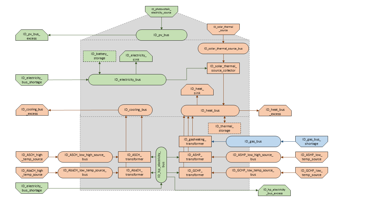
None |
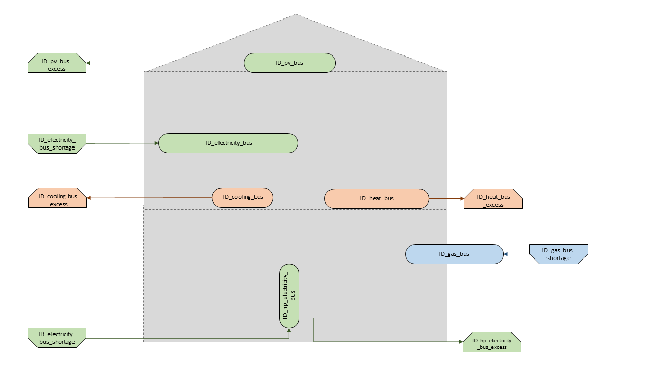
Graph of the energy system, which is created by entering the example components. The non-active components are not included in the graph above.
District Heating
Within this sheet, the road network structure of the energy system is defined. The following parameters need to be entered:
label: Unique designation of the street section, e.g. the street section name. Also for streets that are not activated.
comment: Space for an individual comment.
active: Specifies whether the street section shall be included to the model. “0” = inactive, “1” = active.
lat. 1st intersection: Latitude (WGS84) of the first point of the given street part.
lon. 1st intersection: Longitude (WGS84) of the first point of the given street part.
lat. 2nd intersection: Latitude (WGS84) of the second point of the given street part.
lon. 2nd intersection: Longitude (WGS84) of the second point of the given street part.
label |
comment |
active |
lat. 1st intersection |
lat. 2nd intersection |
lat. 1st intersection |
lon. 2nd intersection |
|---|---|---|---|---|---|---|
ID_street1 |
1 |
45.00 |
55.00 |
5.00 |
10.00 |
Sinks
Within this sheet, the sinks of the energy system are defined. The following parameters need to be entered:
label: Unique designation of the sink. Also for sinks that are not activated. The following format is recommended: “<ID>_<energy sector>_sink”. <ID> and <energy sector> need to be replaced by the sink attributes.
comment: Space for an individual comment, e.g. an indication of which measure this component belongs to.
active: Specifies whether the sink shall be included to the model. “0” = inactive, “1” = active.
fixed: Specifies whether it is a fixed sink or not. “0” = not fixed; “1” = fixed.
input: Specifies the bus from which the input to the sink comes from.
load profile: Specifies the basis onto which the load profile of the sink is to be created. If the Richardson tool is to be used, “richardson” has to be inserted. For standard load profiles, its acronym is used. The different load profiles are explained here. If a time series is used, “timeseries” must be entered and must be provided in the Time series sheet. If the sink is not fixed, the fill character “x” has to be used.
nominal value in (kW): Nominal performance of the sink. Required when “timeseries” has been entered into the “load profile”. When SLP or Richardson is used, use the fill character “0” here.
annual demand in (kWh/a): Annual energy demand of the sink. Required when using the Richardson Tool or standard load profiles. When using time series, the fill character “0” is used.
occupants [RICHARDSON]: Number of occupants living in the respective building. Only required when using the Richardson tool, use fill character “0” for other load profiles.
building class [HEAT SLP ONLY]: The BDEW building classes are needed for the creating of the non-commercial slp. The parameter building_class (German: Baualtersklasse) can assume values in the range 1-11. The different building classes are explained here (building class 12 was added later and is therefore not available). For non-residential buildings the building class “0” is used.
wind class [HEAT SLP ONLY]: Wind classification for building location (“0” = not windy, “1” = windy).
sector: This column is used to assign the sinks’ energy amounts to the energy amount diagrams in the result processing. Possible entries: electricity, heat, cooling.
label |
comment |
active |
fixed |
input |
load profile |
nominal value |
annual demand |
occupants |
building class |
wind class |
sector |
|---|---|---|---|---|---|---|---|---|---|---|---|
(kW) |
(kWh/a) |
(richardson) |
(heat slp) |
(heat slp) |
|||||||
ID_electricity_sink |
1 |
1 |
ID_electricity_bus |
h0 |
0 |
5000.0 |
0 |
0 |
0 |
electricity |
|
ID_heat_sink |
1 |
1 |
ID_heat_bus |
efh |
0 |
30000.0 |
0 |
3 |
0 |
heat |
|
ID_cooling_sink |
0 |
1 |
ID_cooling_bus |
timeseries |
1 |
0 |
0 |
0 |
0 |
cooling |
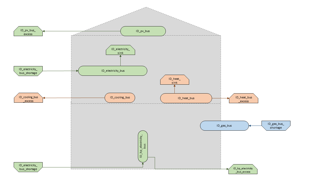
Graph of the energy system, which is created by entering the example components. The non-active components are not included in the graph above.
Sources
Within this sheet, the sources of the energy system are defined. Technology specific data (see 2nd line), must be filled in only if the respective technology is selected otherwise use “0”. The following parameters have to be entered:
label: Unique designation of the source. Also for sources that are not activated. The following format is recommended: “<ID>_<energy sector>_source”. <ID> and <energy sector> need to be replaced by the bus attributes.
comment: Space for an individual comment, e.g. an indication of which measure this component belongs to.
active: Specifies whether the source shall be included to the model. “0” = inactive, “1” = active.
fixed: Indicates whether it is a fixed source or not. “0” = not fixed; “1” = fixed.
output: Specifies which bus the output of the source is connected to.
input: Specifies which bus the input of the source is connected to (currently not required for any technology).
technology: Technology type of source. Input options: “photovoltaic”, “windpower”, “timeseries”, “other”, “solar_thermal_flat_plate”, “concentrated_solar_power”. Time series are automatically generated for photovoltaic systems and wind turbines. If “timeseries” is selected, a time series must be provided in the Time series sheet.
sector: This column is used to differentiate between an electricity, heat and cooling source for the result processing energy amount collection. Possible entries: “electricity”, “heat”, “cooling”, “central_electricity”, “central_heat”, “central_cooling”.
Costs
existing capacity in (kW): Existing capacity of the source before possible investment.
min. investment capacity in (kW): Minimum capacity to be installed in case of an investment.
max. investment capacity in (kW): Maximum capacity that can be added in the case of an investment. If no investment is possible, enter the value “0” here.
variable costs in (CU/kWh): Defines the variable costs incurred for a kWh of energy drawn from the source.
variable constraint costs in (CU/kWh): Defines the variable costs incurred for a kWh of energy drawn from the source referring to the constraint limit set in the “energysystem” sheet. If not considering constraints fill character “0” is used.
periodical costs in (CU/(kW a)): Costs incurred per kW for investments within the time horizon. Periodical costs only apply for newly invested capacities but not for existing capacities.
periodical constraint costs in (CU/(kW a)): Costs incurred per kW for investments within the time horizon referring to the constraint limit set in the “energysystem” sheet. If not considering constraints fill character “0” is used.
non-convex investment: Specifies whether the investment capacity should be defined as a mixed-integer variable, i.e. whether the model can decide whether NOTHING OR THE INVESTMENT should be implemented. Explained here.
fix investment costs in (CU/a): Fixed costs of non-convex investments (in addition to the periodic costs).
fix investment constraint costs in (CU/a): Fixed constraint costs of non-convex investments (in addition to the periodic constraint costs).
Wind
The following parameters need to be set for wind power sources.
The wind speed timeseries entered in the Weather data sheet (measured at 10 m height) will get converted into wind speeds at specified hub height. With the specified turbine model an energy timeseries will then be calculated.
Turbine Model: Reference wind turbine model. Possible turbine types are listed in the windpowerlib’s database. Write the value of the column “turbine_type” of the .csv in your spreadsheet.
Hub Height: Hub height of the wind turbine. Which hub heights are possible for the selected reference turbine can be viewed in the windpowerlib’s database too.
PV
The parameters for PV sources depend on the selected technology.
General PV Parameters
Azimuth: Specifies the orientation of the PV module in degrees. Values between “0” and “360” are permissible (“0” = north, “90” = east, “180” = south, “270” = west). Use fill character “0” for other technologies.
Surface Tilt: Specifies the inclination of the module in degrees (“0” = flat). Use fill character “0” for other technologies.
Albedo: Specifies the albedo value of the reflecting floor surface. Only required for photovoltaic sources, use fill character “0” for other technologies.
Altitude: Height (above mean sea level) in meters of the photovoltaic module. Only required for photovoltaic sources, use fill character “0” for other technologies.
Latitude: Geographic latitude (decimal number in WGS84) of the photovoltaic module. Only required for photovoltaic sources, use fill character “0” for other technologies.
Longitude: Geographic longitude (decimal number in WGS84) of the photovoltaic module. Only required for photovoltaic sources, use fill character “0” for other technologies.
DC AC ratio: Defines the ratio of the DC module capacity to the inverter’s AC rated capacity ($P_{DC} / P_{AC}$). This value is mandatory for all PV configurations to correctly scale the inverter limits. Example: A value of 1.2 means the DC plant capacity is 20% larger than the inverter’s maximum AC output. If you want no undersizing/clipping at all, use 1.0. Only required for photovoltaic sources, use fill character “0” for other technologies.
Module Definition
Depending on your technology choice, define the module via database OR manual datasheet entry:
Option A: Database lookup
Modul Model: Module name, according to the database used (see PVLIB database Sandia or PVLIB database CEC ). Possible Modul Models are presented here. Use fill character “0” for other technologies.
Option B: Manual datasheet
Power STC: Power at Standard Test Conditions (STC) in Watt (e.g. 235). Use fill character “0” for other technologies.
Celltype: Type of the solar cell. Possible entries: “monoSi”, “multiSi”, “polySi”, “cis”, “cigs”, “cdte”, “amorphous”. Use fill character “0” for other technologies.
V mp: Voltage at maximum power point in Volt (e.g. 43). Use fill character “0” for other technologies.
I mp: Current at maximum power point in Ampere (e.g. 5,48). Use fill character “0” for other technologies.
V oc: Open-circuit voltage in Volt (e.g. 51,8). Use fill character “0” for other technologies.
I sc: Short-circuit current in Ampere (e.g. 5,84). Use fill character “0” for other technologies.
Alpha sc: Temperature coefficient of the short-circuit current in A/°C (e.g. 0,00175). Data sheets often specify this in %/°C; it must be converted to an absolute value by dividing the percentage by 100 and multiplying the result by the short-circuit current (i_sc). Use fill character “0” for other technologies.
Beta voc: Temperature coefficient of the open-circuit voltage in V/°C (e.g. -0,124). Data sheets often specify this in %/°C; it must be converted to an absolute value by dividing the percentage by 100 and multiplying the result by the open-circuit voltage (v_oc). Use fill character “0” for other technologies.
Gamma pmp: Temperature coefficient of the maximum power point power in %/°C (e.g., “-0.3”). This value is entered directly as a percentage. Use fill character “0” for other technologies.
Cells in series: Number of solar cells connected in series within one module (e.g. 72). Use fill character “0” for other technologies.
Inverter Definition
Define how the inverter is modeled. This works independently of the chosen module technology:
Option A: Database lookup
Inverter Model: Inverter name, according to the database used. Possible Inverter Models are presented here. If found in the database, only the efficiency characteristics (the efficiency curve) of the inverter are used for the simulation. To prevent artificial clipping or unintended shutdowns in single-module simulations, all lower operational thresholds, such as the startup power threshold ($P_{so}$) or minimum MPPT voltage, are programmatically disabled (set to 0). Meanwhile, the inverter’s capacity limits are programmatically normalized and scaled using the mandatory dc_ac_ratio to match the DC system size. Use fill character “0” for other technologies or if you want to use a constant efficiency instead.
Option B: Constant efficiency fallback
Inverter eta: Nominal inverter efficiency as a decimal fraction (e.g., 0.96 for 96% efficiency). This parameter acts as a fallback and is only evaluated if the specified “Inverter Model” is not found in any database. If used, the system falls back to a simplified PVWatts inverter model. Use fill character “0” for other technologies.
Concentrated Solar Power
The following parameters need to be set for concentrated solar power sources.
Azimuth: Specifies the orientation of the PV module in degrees. Values between “0” and “360” are permissible (“0” = north, “90” = east, “180” = south, “270” = west). Use fill character “0” for other technologies.
Surface Tilt: Specifies the inclination of the module in degrees (“0” = flat). Use fill character “0” for other technologies.
ETA 0: Optical efficiency of the collector. Use fill character “0” for other technologies.
A1 in (1/°): Collector specific linear heat loss coefficient. Use fill character “0” for other technologies.
A2 in (1/°)2: Collector specific quadratic heat loss coefficient. Use fill character “0” for other technologies.
C1 in (W/m2 K): Collector specific thermal loss parameter. Only required for concentrated solar power source, use fill character “0” for other technologies.
C2 in (W/m2 K2): Collector specific thermal loss parameter. Only required for concentrated solar power source, use fill character “0” for other technologies.
Temperature Inlet in (°C): Inlet temperature of the solar heat collector module. Use fill character “0” for other technologies.
Temperature Difference in (°C): Temperature Difference between mean and inlet temperature of the solar heat collector module. Use fill character “0” for other technologies.
Cleanliness: Cleanliness of a parabolic through collector. Only required for Concentrated Solar Power source, use fill character “0” for other technologies.
Peripheral Losses: Heat loss coefficient for losses in the collector’s peripheral system. Use fill character “0” for other technologies.
Exemplary values for concentrated_solar_power technology:
Cleanliness |
ETA 0 |
A1 |
A2 |
C1 |
C2 |
|---|---|---|---|---|---|
solar heat |
solar heat |
solar heat |
solar heat |
solar heat |
solar heat |
0.9 |
0.816 |
-0.00159 |
0.0000977 |
0.0622 |
0.00023 |
Solar Thermal Flat Plate
The following parameters need to be set for solar thermal flat plate sources.
Azimuth: Specifies the orientation of the PV module in degrees. Values between “0” and “360” are permissible (“0” = north, “90” = east, “180” = south, “270” = west). Use fill character “0” for other technologies.
Surface Tilt: Specifies the inclination of the module in degrees (“0” = flat). Use fill character “0” for other technologies.
ETA 0: Optical efficiency of the collector. Use fill character “0” for other technologies.
A1 in (1/°): Collector specific linear heat loss coefficient. Use fill character “0” for other technologies.
A2 in (1/°)2: Collector specific quadratic heat loss coefficient. Use fill character “0” for other technologies.
Temperature Inlet in (°C): Inlet temperature of the solar heat collector module. Use fill character “0” for other technologies.
Temperature Difference in (°C): Temperature Difference between mean and inlet temperature of the solar heat collector module. Use fill character “0” for other technologies.
Peripheral Losses: Heat loss coefficient for losses in the collector’s peripheral system. Use fill character “0” for other technologies.
Conversion Factor in (m2 /kW): The factor is explained here.
Timeseries
If you have chosen the technology “timeseries” (in the technology column), you have to include a timeseries in the Time series sheet or use default one.
Commodity
If you have chosen the technology “other” (in the technology column), a commodity source with maximum investable capacity but completely variable time series becomes part of the energy system. The solver can thus design a completely linear source and use it to cover the demand when required.
label |
comment |
active |
fixed |
technology |
output |
input |
existing capacity |
min. investment capacity |
max. investment capapcity |
non-convex investment |
fix investment costs |
variable costs |
periodical costs |
variable constraint costs |
periodical constraint costs |
Turbine Model |
Hub Height |
Modul Model |
Inverter Model |
DC AC Ratio |
Inverter Eta |
Albedo |
Altitude |
Azimuth |
Surface Tilt |
Latitude |
Longitude |
ETA 0 |
A1 |
A2 |
C1 |
C2 |
Temperature Inlet |
Temperature Difference |
Conversion Factor |
Peripheral Losses |
Cleanliness |
power stc |
celltype |
v mp |
i mp |
v oc |
i sc |
alpha sc |
beta voc |
gamma pmp |
cells in series |
sector |
|
|---|---|---|---|---|---|---|---|---|---|---|---|---|---|---|---|---|---|---|---|---|---|---|---|---|---|---|---|---|---|---|---|---|---|---|---|---|---|---|---|---|---|---|---|---|---|---|---|---|---|
solar heat |
(kW) |
(kW) |
(kW) |
(CU/a) |
(CU/kWh) |
(CU/(kW a)) |
(CU/kWh) |
(CU/(kW a)) |
windpower |
windpower |
PV |
PV |
PV |
PV |
PV |
(m) | PV |
(°) |
(°) |
(°) |
(°) |
solar heat |
(1/°) | solar heat |
(1/°)2 | solar heat |
(W/m2 K) | solar heat |
(W/m2 K2) | solar heat |
(°C) | solar heat |
(°C) | solar heat |
(m2/kW) | solar heat |
solar heat |
solar heat |
solar heat |
(W) | PV |
PV |
(V) | PV |
(A) | PV |
(V) | PV |
(A) | PV |
(A/°C) | PV |
(V/°C) | PV |
(%/°C) | PV |
PV |
||||||||
ID_photovoltaic_electricity_source |
1 |
1 |
photovoltaic |
ID_pv_bus |
None |
0 |
0 |
20 |
0 |
0 |
0 |
90 |
56 |
0 |
0 |
0 |
Panasonic_VBHN235SA06B__2013_ |
ABB__MICRO_0_25_I_OUTD_US_240__240V_ |
1 |
0 |
0.18 |
60 |
180 |
35 |
52.13 |
7.36 |
0 |
0 |
0 |
0 |
0 |
0 |
0 |
0 |
0 |
0 |
0 |
0 |
0 |
0 |
0 |
0 |
0 |
0 |
0 |
0 |
electricity |
||
ID_solar_thermal_source |
1 |
1 |
solar_thermal_flat_plate |
ID_heat_bus |
ID_electricity_bus |
0 |
0 |
20 |
0 |
0 |
0 |
40 |
25 |
0 |
0 |
0 |
0 |
0 |
0 |
0 |
0 |
0 |
20 |
10 |
52.13 |
7.36 |
0.719 |
1.063 |
0.005 |
0 |
0 |
40 |
15 |
1.79 |
0.05 |
0 |
0 |
0 |
0 |
0 |
0 |
0 |
0 |
0 |
0 |
0 |
heat |
||
wind_turbine |
0 |
1 |
windpower |
electricity_bus |
None |
0 |
0 |
30 |
0 |
0 |
0 |
100 |
9 |
0 |
E-126/4200 |
135 |
0 |
0 |
0 |
0 |
0 |
0 |
0 |
0 |
0 |
0 |
0 |
0 |
0 |
0 |
0 |
0 |
0 |
0 |
0 |
0 |
0 |
0 |
0 |
0 |
0 |
0 |
0 |
0 |
0 |
0 |
electricity |
||
ID_photovoltaic_electricity_source |
1 |
1 |
photovoltaic_datasheet |
ID_pv_bus |
None |
0 |
0 |
20 |
0 |
0 |
0 |
90 |
56 |
0 |
0 |
0 |
0 |
0 |
1 |
0.97 |
0.18 |
60 |
180 |
35 |
52.13 |
7.36 |
0 |
0 |
0 |
0 |
0 |
0 |
0 |
0 |
0 |
0 |
235 |
monoSi |
43 |
5.48 |
51.8 |
5.84 |
0.00175 |
-0.124 |
-0.3 |
72 |
electricity |
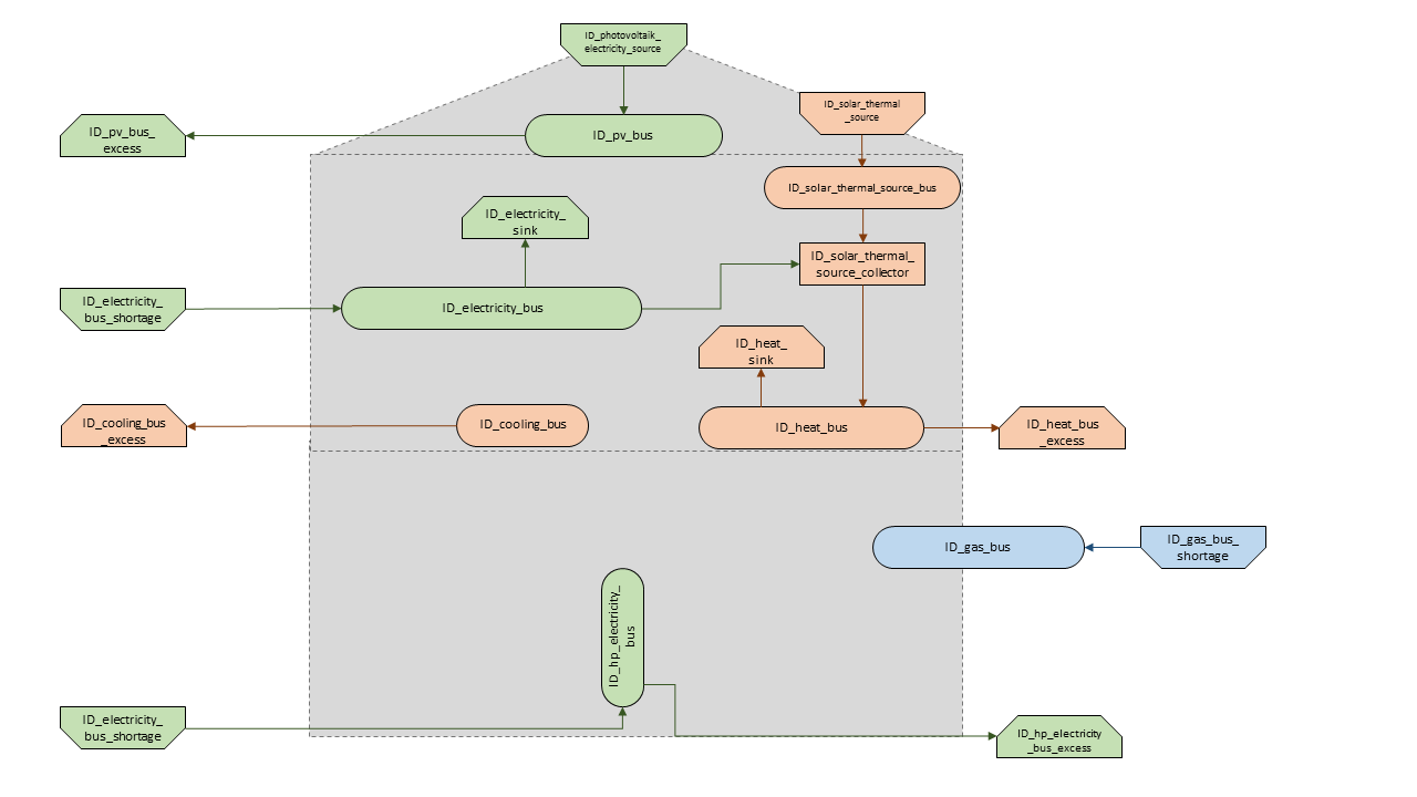
Graph of the energy system, which is created by entering the example components of sources sheet. The non-active components are not included in the graph above.
Transformers
Within this sheet, the transformers of the energy system are defined.
The following parameters have to be entered:
label: Unique designation of the transformer. Also for transformers that are not activated. The following format is recommended: “<ID>_<energy sector>_transformer”. <ID> and <energy sector> need to be replaced by the transformer attributes.
comment: Space for an individual comment, e.g. an indication of which measure this component belongs to.
active: Specifies whether the transformer shall be included to the model. “0” = inactive, “1” = active.
transformer type: Indicates what kind of transformer it is. Possible entries: “GenericTransformer” for linear transformers with constant efficiencies; “GenericTwoInputTransformer” for transformers with two inputs and constant efficiencies (e. g. Pumping units with water and electricity intake); “GenericCHP” for transformers with varying efficiencies; “CompressionHeatTransformer”; “AbsorptionHeatTransformer”.
mode: Specifies, if a compression or absorption heat transformer is working as “chiller” or “heat_pump”. Only required if “transformer type” is set to “CompressionHeatTransformer” or “AbsorptionHeatTransformer”. Otherwise has to be set to “0”.
input: Specifies the bus from which the input to the transformer comes from.
input2: Specifies the bus from which the secondary input of the transformer comes from. Only required if “transformer type” is set to “GenericTwoInputTransformer”. If there is no second input, the fill character “0” must be entered here.
output: Specifies bus to which the output of the transformer is forwarded to. If the sector “central_heat” is selected for a CHP the electrical output bus must be used here. If the sector “central_electricity” is selected for a CHP the heat output bus must be used here.
output2: Specifies the bus to which the secondary output of the transformer is forwarded to. If there is no second output, the fill character “0” must be entered here.
input2 / input: Specifies the ratio of input2 to input (e.g. kWh/m3). The ratio is further used to calculate to factors for the input flows. If a transformer uses two inputs of the same types with different amounts this can also be considered with the ratio (e.g. 60% biogas and 40% naturalgas can be translated to a ratio of 0,6/0,4=1,25). Only required if “transformer type” is set to “GenericTwoInputTransformer”. If there is no second input, the fill character “0” must be entered here.
sector: This column is used to differentiate the transformer types for the result processing energy amount collection. Possible entries: “electricity”, “heat”, “cooling”, “central_electricity”, “central_heat”, “central_cooling”, “electric_heating”.
technology: The technology column represents the category in which the energy quantities for the energy quantity diagrams are collected. If, for example, “natural_gasheating” is entered for a component, it will appear under natural_gasheating in the energy quantity diagram. Attention: If in the sector “central_”… is used in the sector, a leading “central_” is appended to the selected technology in the balancing.
Costs
existing capacity in (kW): Existing capacity of the transformer before possible investment.
min investment capacity in (kW): Minimum transformer capacity to be installed.
max investment capacity in (kW): Maximum installable transformer capacity regarding the output of the transformer, in addition to previously installed capacity, if existing.
variable input costs in (CU/kWh): Variable costs incurred per kWh of input energy supplied.
variable input costs 2 in (CU/kWh): Variable costs incurred per kWh of input 2 energy supplied.
variable output costs in (CU/kWh): Variable costs incurred per kWh of output energy supplied.
variable output costs 2 in (CU/kWh): Variable costs incurred per kWh of output 2 energy supplied.
variable input constraint costs in (CU/kWh): Variable constraint costs incurred per kWh of input energy supplied referring to the constraint limit set in the “energysystem” sheet. If not considering constraints fill character “0” is used.
variable input constraint costs 2 in (CU/kWh): Variable constraint costs incurred per kWh of input2 energy supplied referring to the constraint limit set in the “energysystem” sheet. If not considering constraints fill character “0” is used.
variable output constraint costs in (CU/kWh): Variable constraint costs incurred per kWh of output energy supplied referring to the constraint limit set in the “energysystem” sheet. If not considering constraints fill character “0” is used.
variable output constraint costs 2 in (CU/kWh): Variable constraint costs incurred per kWh of output 2 energy supplied referring to the constraint limit set in the “energysystem” sheet. If not considering constraints fill character “0” is used.
periodical costs in (CU/a): Costs incurred per kW for investments within the time horizon. Periodical costs only apply for newly invested capacities but not for existing capacities.
periodical constraint costs in (CU/(kW a)): Constraint costs incurred per kW for investments within the time horizon. If not considering constraints fill character “0” is used.
non-convex investment: Specifies whether the investment capacity should be defined as a mixed-integer variable, i.e. whether the model can decide whether NOTHING OR THE INVESTMENT should be implemented. Explained here.
fix investment costs in (CU/a): Fixed costs of non-convex investments (in addition to the periodic costs).
fix investment constraint costs in (CU/a): Fixed constraint costs of non-convex investments (in addition to the periodic constraint costs).
Generic Transformer
efficiency: Specifies the efficiency of the first output. Values between “0” and “1” are allowed entries.
efficiency2: Specifies the efficiency of the second output, if there is one. Values between “0” and “1” are entered. If there is no second output, the fill character “0” must be entered here.
Compression Heat Transformer
The following parameters are only required, if “transformer type” is set to “CompressionHeatTransformer”:
heat source: Specifies the heat source. Possible heat sources are “GroundWater”, “Ground”, “Air”, “Air-to-Air” (which represents an AAHP) and “Water”.
temperature high in (°C): Temperature of the high temperature heat reservoir. Only required if “mode” is set to “heat_pump”.
temperature low in (°C): Cooling temperature needed for cooling demand. Only required if “mode” is set to “chiller”.
quality grade: To determine the COP of a real machine a scale-down factor (the quality grade) is applied on the Carnot efficiency (see oemof.thermal).
area in (m2): Open spaces for ground-coupled compression heat transformers (GCHP).
length of the geoth. probe in (m): Length of the vertical heat exchanger, only for GCHP.
heat extraction in (kW/(m a)): Heat extraction for the heat exchanger referring to the location, only for GCHP.
min. borehole area in (m2): Limited space due to the regeneration of the ground source, only for GCHP.
temp threshold icing: Temperature below which icing occurs (see oemof.thermal). Only required if “mode” is set to “heat_pump”.
factor icing: Factor to which the COP is reduced caused by icing (e.g. “0.8” if you have a reduction of 20%) (see oemof.thermal). Only required if “mode” is set to “heat_pump”.
Absorption Heat Transformer
The following parameters are only required, if “transformer type” is set to “AbsorptionHeatTransformer”:
name: Defines the way of calculating the efficiency of the absorption heat transformer. Possible inputs are: “Rotartica”, “Safarik”, “Broad_01”, “Broad_02”, and “Kuehn”. “Broad_02” refers to a double-effect absorption chiller model, whereas the other keys refer to single-effect absorption chiller models.
temperature high in (°C): Temperature of the heat source, that drives the absorption heat transformer.
temperature low in (°C): Output temperature which is needed for the cooling demand.
electrical input conversion factor: Specifies the relation of electricity consumption to energy input. Example: A value of “0,05” means, that the system consumes 5 % of the input energy as electric energy.
recooling temperature difference in (°C): Defines the temperature difference between temperature source for recooling and recooling cycle.
heat capacity of source: Defines the heat capacity of the connected heat source e.g. extracted waste heat.
GenericCHP
Warning
Currently the GenericCHP component can only be used for the purpose of simulation. The solver is not able to dimension the components capacity. Since there is no investment decision no periodical costs apply.
min. share of flue gas loss: Percentage flue gas losses of the operating point with maximum heat extraction.
max. share of flue gas loss: Percentage flue gas losses of the operating point with minimum heat extraction.
min. electric power in (kW): Minimum electrical power supply without heat extraction (district heating).
max. electric power in (kW): Maximum electrical power supply without heat extraction (district heating).
min. electric efficiency: Specifies the minimum electric efficiency without heat extraction (district heating). Values between “0” and “1” are allowed entries.
max. electric efficiency: Specifies the minimum electric efficiency without heat extraction (district heating). Values between 0 and 1 are allowed entries.
minimal thermal output power in (kW): Heat output taken from the exhaust gas via a condenser even in purely electric operation.
electric power loss index: Reduction of the electrical power by “electric power loss index * extracted thermal power”.
back pressure: Defines rather the end pressure of “Turbine CHP” is higher than ambient pressure (input value has to be “1”) or not (input value has to be “0”). For “Motoric CHP” it has to be “0”.
label |
comment |
active |
transformer type |
mode |
input |
input2 |
output |
output2 |
input2 / input |
efficiency |
efficiency2 |
existing capacity |
min. investment capacity |
max. investment capacity |
non-convex investment |
fix investment costs |
variable input costs |
variable input costs 2 |
variable output costs |
variable output costs 2 |
periodical costs |
variable input constraint costs |
variable input constraint costs 2 |
variable output constraint costs |
variable output constraint costs 2 |
periodical constraint costs |
heat source |
temperature high |
temperature low |
quality grade |
area |
length of the geoth. probe |
heat extraction |
min. borehole area |
temp. threshold icing |
factor icing |
name |
electrical input conversion factor |
recooling temperature difference |
min. share of flue gas loss |
max. share of flue gas loss |
min. electric power |
max. electric power |
min. electric efficiency |
max. electric efficiency |
minimal thermal output power |
elec. power loss index |
back pressure |
sector |
technology |
|---|---|---|---|---|---|---|---|---|---|---|---|---|---|---|---|---|---|---|---|---|---|---|---|---|---|---|---|---|---|---|---|---|---|---|---|---|---|---|---|---|---|---|---|---|---|---|---|---|---|---|
(kW) |
(kW) |
(kW) |
(CU/a) |
(CU/kWh) |
(CU/kWh) |
(CU/kWh) |
(CU/kWh) |
(CU/(kW a)) |
(CU/kWh) |
(CU/kWh) |
(CU/kWh) |
(CU/kWh) |
(CU/(kW a)) |
(°C) |
(°C) |
(m2) |
(m) |
(kW/(m a)) |
(m2) |
(°C) |
(°C) |
(kW) |
(kW) |
(kW) |
||||||||||||||||||||||||||
ID_gasheating_transformer |
1 |
GenericTransformer |
0 |
ID_gas_bus |
0 |
ID_heat_bus |
0 |
0 |
0.85 |
0 |
0 |
0 |
20 |
0 |
0 |
0 |
0 |
0 |
0 |
70 |
0 |
0 |
200 |
0 |
0 |
0 |
0 |
0 |
0 |
0 |
0 |
0 |
0 |
0 |
0 |
0 |
0 |
0 |
0 |
0 |
0 |
0 |
0 |
0 |
0 |
0 |
0 |
heat |
natural_gasheating |
|
ID_TwoInput_transformer |
0 |
GenericTwoInputTransformer |
0 |
ID_water_intake_bus |
ID_electricity_intake_bus |
ID_water_output_bus |
0 |
0.84 |
0.88 |
0 |
0 |
0 |
20 |
0 |
0 |
0 |
0 |
0 |
0 |
6.600 |
0 |
0 |
0 |
0 |
0 |
0 |
0 |
0 |
0 |
0 |
0 |
0 |
0 |
0 |
0 |
0 |
0 |
0 |
0 |
0 |
0 |
0 |
0 |
0 |
0 |
0 |
0 |
None |
None |
|
ID_GCHP_transformer |
1 |
CompressionHeatTransformer |
heat_pump |
ID_hp_electricity_bus |
0 |
ID_heat_bus |
0 |
0 |
1 |
0 |
0 |
0 |
20 |
0 |
0 |
0 |
0 |
0 |
0 |
115.57 |
0 |
0 |
0 |
0 |
0 |
Ground |
60 |
0 |
0.6 |
1000 |
100 |
0.05 |
100 |
3 |
0.8 |
0 |
0 |
0 |
0 |
0 |
0 |
0 |
0 |
0 |
0 |
0 |
0 |
heat |
GCHP |
|
ID_ASCH_transformer |
1 |
CompressionHeatTransformer |
chiller |
ID_hp_electricity_bus |
0 |
ID_cooling_bus |
0 |
0 |
1 |
0 |
0 |
0 |
20 |
0 |
0 |
0 |
0 |
0 |
0 |
100 |
0 |
0 |
0 |
0 |
0 |
Air |
0 |
-10 |
0.4 |
0 |
0 |
0 |
0 |
0 |
0 |
0 |
0 |
0 |
0 |
0 |
0 |
0 |
0 |
0 |
0 |
0 |
0 |
cooling |
ASCH |
|
ID_AbsCH_transformer |
1 |
AbsorptionHeatTransformer |
chiller |
ID_hp_electricity_bus |
0 |
ID_cooling_bus |
0 |
0 |
1 |
0 |
0 |
0 |
20 |
0 |
0 |
0 |
0 |
0 |
0 |
100 |
0 |
0 |
0 |
0 |
0 |
0 |
85 |
10 |
0 |
0 |
0 |
0 |
0 |
0 |
0 |
Kuehn |
0.05 |
6 |
0 |
0 |
0 |
0 |
0 |
0 |
0 |
0 |
0 |
cooling |
AbsCH |
|
ID_ASHP_transformer |
1 |
CompressionHeatTransformer |
heat_pump |
ID_hp_electricity_bus |
0 |
ID_heat_bus |
0 |
0 |
1 |
0 |
0 |
0 |
20 |
0 |
0 |
0 |
0 |
0 |
0 |
112.78 |
0 |
0 |
0 |
0 |
0 |
Air |
60 |
0 |
0.4 |
0 |
0 |
0 |
0 |
3 |
0.8 |
0 |
0 |
0 |
0 |
0 |
0 |
0 |
0 |
0 |
0 |
0 |
0 |
heat |
ASHP |
|
ID_chp_transformer |
0 |
GenericTransformer |
0 |
district_gas_bus |
0 |
district_chp_electricity_bus |
district_heat_bus |
0 |
0.35 |
0.55 |
0 |
0 |
20 |
0 |
0 |
0 |
0 |
0 |
0 |
50 |
130 |
0 |
375 |
0 |
0 |
0 |
0 |
0 |
0 |
0 |
0 |
0 |
0 |
0 |
0 |
0 |
0 |
0 |
0 |
0 |
0 |
0 |
0 |
0 |
0 |
0 |
0 |
heat |
natural_gas_CHP |
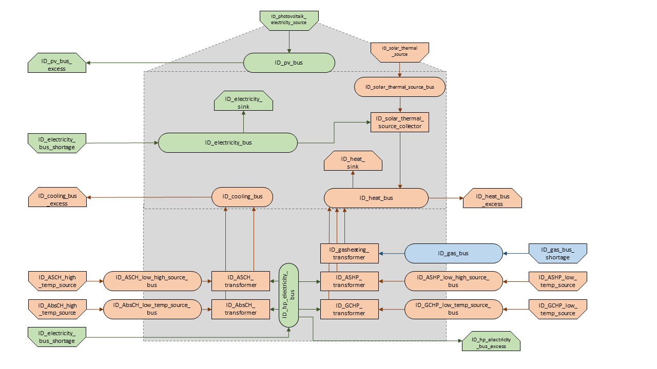
Graph of the energy system, which is created by entering the example components. The non-active components are not included in the graph above.
Storages
Within this sheet, the storages of the energy system are defined. The following parameters have to be entered:
label: Unique designation of the storage. Also for storages that are not activated. The following format is recommended: “<ID>_<energy sector>_storage”. <ID> and <energy sector> need to be replaced by the storage attributes.
comment: Space for an individual comment, e.g. an indication of which measure this component belongs to.
active: Specifies whether the storage shall be included to the model. “0” = inactive, “1” = active.
storage type: Defines whether the storage is a “Generic” or a “Stratified” storage. These two inputs are possible.
input: Specifies the input of the storage. If the storage has only one connection, the same bus can be provided for input and output.
output: Specifies the output of the storage. If the storage has only one connection, the same bus can be provided for input and output.
input/capacity ratio (invest): Indicates the performance with which the storage can be charged (see also here).
output/capacity ratio (invest): Indicates the performance with which the storage can be discharged (see also here).
efficiency inflow: Specifies the charging efficiency.
efficiency outflow: Specifies the discharging efficiency.
initial capacity: Specifies how far the storage is loaded at time 0 of the simulation. Value must be between “0” and “1”. The initial capacity value must be equal or higher than the ‘capacity min’ value.
capacity min: Specifies the minimum amount of storage that must be loaded at any given time. Value must be between “0” and “1”.
capacity max: Specifies the maximum amount of storage that can be loaded at any given time. Value must be between “0” and “1”.
sector: This column is used to differentiate between an electricity, heat and cooling storages for the result processing energy amount collection. Possible entries: “electricity”, “heat”, “cooling”, “central_electricity”, “central_heat”, “central_cooling”.
Costs
existing capacity in (kW): Existing capacity of the storage before possible investment.
min. investment capacity in (kW): Minimum storage capacity to be installed.
max. investment capacity in (kW): Maximum in addition to existing capacity, installable storage capacity.
variable input costs in (CU/kWh): Indicates how many costs arise for charging with one kWh.
variable output costs in (CU/kWh): Indicates how many costs arise for charging with one kWh.
variable input constraint costs in (CU/kWh): Indicates how many costs arise for charging with one kWh referring to the constraint limit set in the “energysystem” sheet. If not considering constraints fill character “0” is used.
variable output constraint costs in (CU/kWh): Indicates how many costs arise for charging with one kWh referring to the constraint limit set in the “energysystem” sheet. If not considering constraints fill character “0” is used.
periodical costs in (CU/a): Costs incurred per kW for investments within the time horizon. Periodical costs only apply for newly invested capacities but not for existing capacities.
periodical constraint costs in (CU/a): Costs incurred per kW for investments within the time horizon referring to the constraint limit set in the “energysystem” sheet. If not considering constraints fill character “0” is used.
non-convex investment: Specifies whether the investment capacity should be defined as a mixed-integer variable, i.e. whether the model can decide whether NOTHING OR THE INVESTMENT should be implemented. Explained here.
fix investment costs in (CU/a): Fixed costs of non-convex investments (in addition to the periodic costs).
fix investment constraint costs in (CU/a): Fixed constraint costs of non-convex investments (in addition to the periodic costs).
Generic Storage
capacity loss: Indicates the storage loss per time unit where “0,03” represents 3 % daily losses. Only required, if the “storage type” is set to “Generic”.
Stratified Storage
diameter in (m): Defines the diameter of a stratified thermal storage, which is necessary for the calculation of thermal losses.
temperature high in (°C): Outlet temperature of the stratified thermal storage.
temperature low in (°C): Inlet temperature of the stratified thermal storage.
U value in (W/(m2 K)): Thermal transmittance coefficient.
label |
comment |
active |
storage type |
bus |
input/capacity ratio |
output/capacity ratio |
efficiency inflow |
efficiency outflow |
initial capacity |
capacity min |
capacity max |
existing capacity |
min. investment capacity |
max. investment capacity |
non-convex investment |
fix investment costs |
variable input costs |
variable output costs |
periodical costs |
variable input constraint costs |
variable output constraint costs |
periodical constraint costs |
capacity loss |
diameter |
temperature high |
temperature low |
U value |
sector |
|---|---|---|---|---|---|---|---|---|---|---|---|---|---|---|---|---|---|---|---|---|---|---|---|---|---|---|---|---|
(invest) |
(invest) |
(kWh) |
(kWh) |
(kWh) |
(CU/a) |
(CU/kWh) |
(CU/kWh) |
(CU/(kWh a)) |
(CU/kWh) |
(CU/kWh) |
(CU/(kWh a)) |
Generic Storage |
(m) | Stratified Storage |
(°C) | Stratified Storage |
Stratified Storage |
(W/(m2 K)) | Stratified Storage |
||||||||||||
ID_battery_storage |
1 |
Generic |
ID_electricity_bus |
0.17 |
0.17 |
1 |
0.98 |
0.1 |
0.1 |
1 |
0 |
0 |
100 |
0 |
0 |
0 |
0 |
70 |
0 |
0 |
400 |
0 |
0 |
0 |
0 |
0 |
electricity |
|
ID_thermal_storage |
1 |
Generic |
ID_heat_bus |
0.17 |
0.17 |
1 |
0.98 |
0.1 |
0.1 |
0.9 |
0 |
0 |
100 |
0 |
0 |
0 |
20 |
35 |
0 |
0 |
100 |
0 |
0 |
0 |
0 |
0 |
heat |
|
ID_stratified_thermal_storage |
0 |
Stratified |
ID_heat_bus |
0.2 |
0.2 |
1 |
0.98 |
0.05 |
0.05 |
0.95 |
0 |
0 |
100 |
0 |
0 |
0 |
20 |
35 |
0 |
0 |
100 |
0 |
0.8 |
60 |
40 |
0.04 |
heat |
|
district_battery_storage |
0 |
Generic |
district_electricity_bus |
0.17 |
0.17 |
1 |
0.98 |
0.1 |
0.1 |
1 |
0 |
0 |
1000 |
0 |
0 |
0 |
0 |
10 |
0 |
0 |
10 |
0 |
0 |
0 |
0 |
0 |
central_electricity |
Graph of the energy system, which is created after entering the example components. The non-active components are not included in the graph above.
Links
Within this sheet, the links of the energy system are defined. The following parameters have to be entered:
label: Unique designation of the link. Also for links that are not activated. The following format is recommended: “<ID>_<energy sector>_link”. <ID> and <energy sector> need to be replaced by the link attributes.
comment: Space for an individual comment, e.g. an indication of which measure this component belongs to.
active: Specifies whether the link shall be included to the model. “0” = inactive, “1” = active.
bus1: First bus to which the link is connected. If it is a directed link, this is the input bus.
bus2: Second bus to which the link is connected. If it is a directed link, this is the output bus.
(un)directed: Specifies whether it is a directed or an undirected link. Input options: “directed”, “undirected”.
efficiency: Specifies the efficiency of the link. Values between 0 and 1 are allowed entries.
timeseries: Specifies whether the maximum transport capacity is limited by a timeseries in the Time series sheet or not. “0” = no timeseries, “1” = timeseries
Costs
existing capacity in (kW): Existing capacity of the link before possible investment.
min. investment capacity in (kW): Minimum, in addition to existing capacity, installable capacity.
max. investment capacity in (kW): Maximum capacity to be installed.
variable output costs in (CU/kWh): Indicates how many costs arise for transporting one kWh.
variable output constraint costs in (CU/kWh): Constraint costs incurred per kWh referring to the constraint limit set in the “energysystem” sheet. If not considering constraints fill character “0” is used.
periodical costs in (CU/(kW a)): Costs incurred per kW for investments within the time horizon. Periodical costs only apply for newly invested capacities but not for existing capacities.
periodical constraint costs in (CU/(kW a)): Costs incurred per kW for investments within the time horizon referring to the constraint limit set in the “energysystem” sheet. If not considering constraints fill character “0” is used.
non-convex investment: Specifies whether the investment capacity should be defined as a mixed-integer variable, i.e. whether the model can decide whether NOTHING OR THE INVESTMENT should be implemented. Explained here.
fix investment costs in (CU/a): Fixed costs of non-convex investments (in addition to the periodic costs).
fix investment constraint costs in (CU/a): Fixed constraint costs of non-convex investments (in addition to the periodic constraint costs).
label |
comment |
active |
timeseries |
(un)directed |
bus1 |
bus2 |
efficiency |
existing capacity |
min. investment capacity |
max. investment capacity |
non-convex investment |
fix investment costs |
variable output costs |
periodical costs |
variable constraint costs |
periodical constraint costs |
|---|---|---|---|---|---|---|---|---|---|---|---|---|---|---|---|---|
(kW) |
(kW) |
(kW) |
(CU/a) |
(CU/kWh) |
(CU/(kW a)) |
(CU/kWh) |
(CU/(kW a)) |
|||||||||
ID_pv_to_ID_electricity_link |
1 |
0 |
directed |
ID_pv_bus |
ID_electricity_bus |
1 |
0 |
0 |
0 |
0 |
0 |
0 |
0 |
0 |
0 |
|
ID_electricity_to_ID_hp_electricity_bus |
1 |
0 |
directed |
ID_electricity_bus |
ID_hp_electricity_bus |
1 |
0 |
0 |
0 |
0 |
0 |
0 |
0 |
0 |
0 |
|
district_heat_directed_link |
0 |
0 |
directed |
district_heat_bus |
ID_heat_bus |
0.85 |
0 |
0 |
0 |
0 |
0 |
0 |
0 |
0 |
0 |
|
district_heat_undirected_link |
0 |
0 |
undirected |
district_heat_bus |
ID_heat_bus |
0.85 |
0 |
0 |
0 |
0 |
0 |
0 |
0 |
0 |
0 |
|
district_electricity_link |
0 |
0 |
directed |
district_electricity_bus |
ID_electricity_bus |
1 |
0 |
0 |
0 |
0 |
0 |
0.1438 |
0 |
0 |
0 |
|
district_chp_to_district_electricity_bus |
0 |
0 |
directed |
district_chp_electricity_bus |
district_electricity_bus |
1 |
0 |
0 |
0 |
0 |
0 |
0.1438 |
0 |
0 |
0 |
|
ID_pv_to_district_electricity_link |
0 |
0 |
directed |
ID_pv_bus |
ID_electricity_bus |
1 |
0 |
0 |
0 |
0 |
0 |
0.1438 |
0 |
0 |
0 |
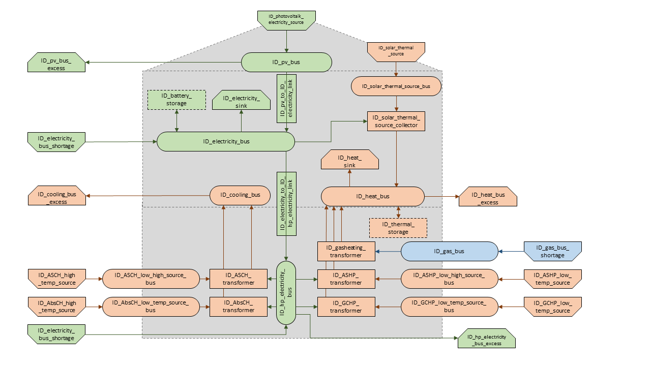
Graph of the energy system, which is created by entering the example components. The non-active components are not included in the graph above.
Insulation
Within this sheet, the energy system insulation options are defined. The following parameters have to be entered:
label: Unique designation of the insulation. Also for insulations that are not activated. The following format is recommended: “<ID>_<sink_label>_<insulation_type>”. <ID>, <sink_label> and <insulation_type> need to be replaced by the insulation attributes.
comment: Space for an individual comment, e.g. an indication of which measure this component belongs to.
active: Specifies whether the insulation shall be included to the model. “0” = inactive, “1” = active.
existing: Existing represents a boolean decision (“0” = no, “1” = yes). If a “1” is filled in here, the insulation measure is completely implemented without incurring any costs.
sink: Sink influenced by the insulation.
temperature indoor in (°C): Definition of the living space temperature.
heat limit temperature in (°C): Temperature from which the heating is switched on.
U-value old in (W/(m2 K)): U-value before insulation.
U-value new in (W/(m2 K)): U-value after insulation.
area in (m2): Area that can be considered for isolation.
periodical costs in (CU/(m2 *a)): Costs incurred per m2 for investments within the time horizon.
periodical constraint costs in (CU/(m2 *a)): Costs incurred per m2 for investments within the time horizon referring to the constraint limit set in the “energysystem” sheet. If not considering constraints fill character “0” is used.
label |
comment |
active |
existing |
sink |
temperature indoor |
heat limit temperature |
U-value old |
U-value new |
area |
periodical costs |
periodical constraint costs |
|---|---|---|---|---|---|---|---|---|---|---|---|
(°C) |
(°C) |
(W/(m2 K)) |
(W/(m2 K)) |
(m2) |
(CU/(m2)) |
(CU/(m2)) |
|||||
ID_heat_sink_window |
1 |
0 |
ID_heat_sink |
20 |
15 |
2.8 |
0.825 |
157.35 |
2400 |
21.9 |
Time Series
Within this sheet, time series and time-dependent price series, are stored. Time series are specified for components for which no automatically generated time series exist. These can be sinks to which the property “load profile” has been assigned as “time series” and sources with the “technology” property “time series”. Time-dependent price series are specified for buses with excess sinks or shortage sources where each period has a different price. These can be buses to which the property “excess costs” or “shortage costs” has been assigned as “timeseries”. The following parameters must be entered:
timestamp: Points in time to which the stored time series are related. The timestamps in the time series refer to local time, allowing the use of real measured data. On the days of the time change, specifically March 28 and October 28, there are special cases. On March 28, the clock is set forward from 2:00 AM to 3:00 AM, which means the hour between 2:00 and 2:59 AM does not exist in local time and is therefore missing in the data. On October 28, the clock is set back from 3:00 AM to 2:00 AM, causing the hour between 2:00 and 2:59 AM to occur twice (for the example of 2012). This results in a duplicated time span in the data for that hour. These effects arise from switching between daylight saving time and standard time. When working with local times, these missing or repeated hours must be taken into account to ensure data consistency. .
timeseries: Time series of a sink or a source which has been assigned the property “timeseries” under the attribute “load profile” or “technology. Time series contain a value between 0 and 1 for each point in time, which indicates the proportion of installed capacity accounted for by the capacity produced at that point in time. In the header line, the name must rather be entered in the format “componentID.fix” if the component enters the power system as a fixed component or it requires two columns in the format “componentID.min” and “componentID.max” if it is an unfixed component. The columns “componentID.min/.max” define the range that the solver can use for its optimization.
price series: Price Series of a bus with excess sink or shortage source which has been assigned the property “timeseries” under the attribute “excess costs” or “shortage costs”. In the header line, the name must be entered in the format “componentID.excess” for buses with excess sinks and “componentID.shortage” for buses with shortage sources. It is possible for a bus to have time-dependent price series in both a excess sink and a shortage source.
timestamp |
residential_electricity_demand.actual_value |
fixed_timeseries_electricty_source.fix |
unfixed_timeseries_electricty_source.min |
unfixed_timeseries_electricty_source.max |
fixed_timeseries_electricity_sink.fix |
unfixed_timeseries_electricity_sink.min |
unfixed_timeseries_electricity_sink.max |
fixed_timeseries_cooling_demand_sink.fix |
bus.excess |
bus.shortage |
|---|---|---|---|---|---|---|---|---|---|---|
2012-01-01 00:00:00 |
0.559061982 |
0.000000 |
0.000000 |
1.000000 |
0.000000 |
0.000000 |
1.000000 |
100 |
-0.1156 |
0.1156 |
2012-01-01 01:00:00 |
0.533606486 |
0.041667 |
0.000000 |
0.500000 |
0.041667 |
0.000000 |
0.500000 |
100 |
-0.1034 |
0.1034 |
2012-01-01 02:00:00 |
0.506058757 |
0.083333 |
0.000000 |
0.333333 |
0.083333 |
0.000000 |
0.333333 |
100 |
-0.09656 |
0.09656 |
2012-01-01 03:00:00 |
0.504140877 |
0.125000 |
0.000000 |
0.250000 |
0.125000 |
0.000000 |
0.250000 |
100 |
-0.09764 |
0.09764 |
2012-01-01 04:00:00 |
0.507104873 |
0.166667 |
0.000000 |
0.200000 |
0.166667 |
0.000000 |
0.200000 |
100 |
-0.09611 |
0.09611 |
2012-01-01 05:00:00 |
0.511376515 |
0.208333 |
0.000000 |
0.166667 |
0.208333 |
0.000000 |
0.166667 |
100 |
-0.10769 |
0.10769 |
2012-01-01 06:00:00 |
0.541801064 |
0.250000 |
0.000000 |
0.142857 |
0.250000 |
0.000000 |
0.142857 |
100 |
-0.12675 |
0.12675 |
2012-01-01 07:00:00 |
0.569261616 |
0.291667 |
0.000000 |
0.125000 |
0.291667 |
0.000000 |
0.125000 |
100 |
-0.13897 |
0.13897 |
2012-01-01 08:00:00 |
0.602998867 |
0.333333 |
0.000000 |
0.111111 |
0.333333 |
0.000000 |
0.111111 |
100 |
-0.13341 |
0.13341 |
2012-01-01 09:00:00 |
0.629064598 |
0.375000 |
0.000000 |
0.100000 |
0.375000 |
0.000000 |
0.100000 |
100 |
-0.12631 |
0.12631 |
Weather Data
If electrical load profiles are simulated with the Richardson tool, heating load profiles with the demandlib or photovoltaic systems with the feedinlib, weather data must be stored here. The weather data time system should be in conformity with the model’s time system, defined in the sheet “timesystem”.
timestamp: Points in time to which the stored weather data are related.
dhi in (W/m2): Diffuse horizontal irradiance.
dni in (W/m2): Direct normal irradiance.
ghi in (W/m2): Global horizontal irradiance.
pressure in (Pa): Air pressure.
temperature in (°C): Air temperature.
windspeed in (m/s): Wind speed, measured at 10 m height.
z0 in (m): Roughness length of the environment.
ground_temp in (°C): Constant ground temperature at 100 m depth.
water_temp in (°C): Varying water temperature of a river depending on the air temperature.
groundwater_temp in (°C): Constant temperature of the ground water at 6 - 10 m depth in North Rhine-Westphalia.
exergy_network_temp in (°C): Temperatur of the exergy network.
anergy_network_temp in (°C): Temperatur of the anergy network.
timestamp |
dhi |
dni |
ghi |
pressure |
temperature |
windspeed |
z0 |
ground_temp |
water_temp |
groundwater_temp |
exergy_network_temp |
anergy_network_temp |
|---|---|---|---|---|---|---|---|---|---|---|---|---|
2012-01-01 00:00:00 |
0.00 |
0.00 |
0.00 |
100672.78 |
10.03 |
5.33 |
0.49 |
13.7 |
14.62 |
13.06 |
90 |
15 |
2012-01-01 01:00:00 |
0.00 |
0.00 |
0.00 |
100678.25 |
10.36 |
5.13 |
0.49 |
13.7 |
14.62 |
13.06 |
90 |
15 |
2012-01-01 02:00:00 |
0.00 |
0.00 |
0.00 |
100680.18 |
10.57 |
4.99 |
0.49 |
13.7 |
14.71 |
13.06 |
90 |
15 |
2012-01-01 03:00:00 |
0.00 |
0.00 |
0.00 |
100651.83 |
10.67 |
4.93 |
0.49 |
13.7 |
14.75 |
13.06 |
90 |
15 |
2012-01-01 04:00:00 |
0.00 |
0.00 |
0.00 |
100618.33 |
10.81 |
4.86 |
0.49 |
13.7 |
14.99 |
13.06 |
90 |
15 |
2012-01-01 05:00:00 |
0.00 |
0.00 |
0.00 |
100594.81 |
10.73 |
5.26 |
0.49 |
13.7 |
14.97 |
13.06 |
90 |
15 |
2012-01-01 06:00:00 |
0.00 |
0.00 |
0.00 |
100558.41 |
10.83 |
5.39 |
0.49 |
13.7 |
14.96 |
13.06 |
90 |
15 |
2012-01-01 07:00:00 |
0.35 |
0.00 |
0.35 |
100566.46 |
11.10 |
5.79 |
0.49 |
13.7 |
15.17 |
13.06 |
90 |
15 |
2012-01-01 08:00:00 |
3.84 |
0.00 |
3.84 |
100572.26 |
11.14 |
5.86 |
0.49 |
13.7 |
15.46 |
13.06 |
90 |
15 |
2012-01-01 09:00:00 |
9.77 |
0.00 |
9.77 |
100568.07 |
11.26 |
5.99 |
0.49 |
13.7 |
15.57 |
13.06 |
90 |
15 |
2012-01-01 10:00:00 |
11.87 |
0.00 |
11.87 |
100560.02 |
11.63 |
5.79 |
0.49 |
13.7 |
15.44 |
13.06 |
90 |
15 |
… |
… |
… |
… |
… |
… |
… |
… |
… |
… |
… |
Pipe Types
Two different components are listed in this table. The first defines the different pipe types available to the energy system for the construction of heating networks and second the components which are the connection between the houses and the heat networks. These are the “dh_heatstation” for the exergy heat network and the “ anergy_heat_pump” for the anergy heat network.
label: Unique designation of the pipe types. Also for pipe types that are not activated. The following format is recommended for the pipes: “<DN>-<diameter of pipe>”.
active: Specifies whether the pipe type shall be included to the model. “0” = inactive, “1” = active.
nonconvex: Specifies whether the investment capacity should be defined as a mixed-integer variable, i.e. whether the model can decide whether NOTHING OR THE INVESTMENT should be implemented. Explained here.
loss factor: Proportional loss factor for the component.
loss factor fix: Fixed loss factor for the component.
min. investment capacity in (kW): Minimum capacity to be installed in case of an investment.
max. investment capacity in (kW): Maximum capacity that can be added in the case of an investment. If no investment is possible, enter the value “0” here.
periodical costs in (CU/(kW a)): Costs incurred per kW for investments within the time horizon. Periodical costs only apply for newly invested capacities but not for existing capacities.
fix investment costs in (CU/a): Fixed costs of non-convex investments (in addition to the periodic costs).
periodical constraint costs in (CU/(kW a)): Costs incurred per kW for investments within the time horizon referring to the constraint limit set in the “energysystem” sheet. If not considering constraints fill character “0” is used.
fix investment constraint costs in (CU/a): Fixed constraint costs of non-convex investments (in addition to the periodic constraint costs).
anergy or exergy: Specifies whether the pipe type is part of the anergy or exergy network. Fill in “exergy” for a pipe for an exergy network and “anergy” for a pipe of an anergy network.
distribution pipe: Specifies whether the pipe type can be used as a distribution pipe. Fill in “1” if the pipe type can be used and “0” if it cannot.
building pipe: Specifies whether the pipe type can be used as a building pipe. Fill in “1” if the pipe type can be used and “0” if it cannot.
efficiency: Specifies the efficiency of the first output. Values between “0” and “1” are allowed entries. This value is only relevant for the “dh_heatstation” and the “anergy_heat_pump”. A “0” can be inserted for the pipe types.
Exemplary input for pipe types label
active
nonconvex
loss factor
loss factor fix
min. investment capacity
max. investment capacity
periodical costs
fix investment costs
periodical constraint costs
fix investment constraint costs
anergy or exergy
distribution pipe
building pipe
efficiency
DN-20
0
1
0
0.010667
0
24.42
0
64
204
0
exergy
1
1
0
DN-25
0
1
0
0.012667
0
43.95
0
65
244
0
exergy
1
1
0
DN-32
0
1
0
0.015333
0
83.44
0
69
304
0
exergy
1
1
0
DN-40
0
1
0
0.017333
0
147.99
0
72
376
0
exergy
1
1
0
DN-50
0
1
0
0.019333
0
261.12
0
81
471.999847
0
exergy
1
1
0
DN-65
0
1
0
0.022
0
506.3
0
88
629
0.00001
exergy
0
1
0
DN-80
0
1
0
0.023333
0
851.92
0
101
800.999977
0.00001
exergy
1
0
0
DN-100
0
1
0
0.026
0
1490
0
125
1056
0
exergy
1
1
0
DN-125
0
1
0
0.028
0
2580
0
150
1412
0
exergy
1
1
0
DN-150
0
1
0
0.029333
0
4050
0
181
1812
0
exergy
1
1
0
DN-200
0
1
0
0.032
0
8220
0
215
2742
0
exergy
1
1
0
DN-250
0
1
0
0.034
0
14210
0
288
3844
0
exergy
1
1
0
Diameter65L
1
0
0.000022
0
0
9999
0.087724
0
0.627025
0
exergy
1
1
0
clustered_consumer_link
1
0
0
0
0
0
0.156558276
0
0.9122902
0
0
0
0
0.02898939
dh_heatstation
1
0
0
0
0
0
85
0
0.000001
0
0
0
0
0.98
anergy_heat_pump
1
0
0
0
0
0
1
0
1
0
0
0
0
1