Application
- The user interface can be used to
create energy system models,
perform optimization and
to process the results.
The basis for any application is the so-called model_definition.xlsx, which can be created either manually or automatically. When creating manually, the model_definition.xlsx must be filled in as described below (see `model definition`_). In case of automatic creation, the Upscaling-Tool (see upscaling tool) is used. After the model_definition.xlsx is filled in, the Main Application (main application) can be started. The structure of the GUI can be seen in the following figure. The sidebar is used to enter input data. The main page is used for descriptions or for displaying results.
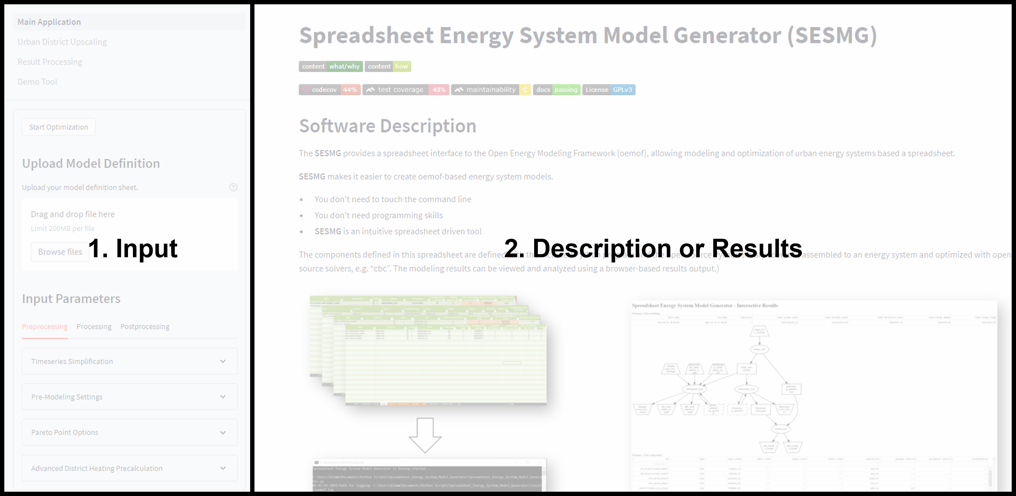
Main Application
The figure shows which steps must be done for optimize an energy system model. At the bottom of the side bar you will find a button that deletes all stored data such as time series reduction values.
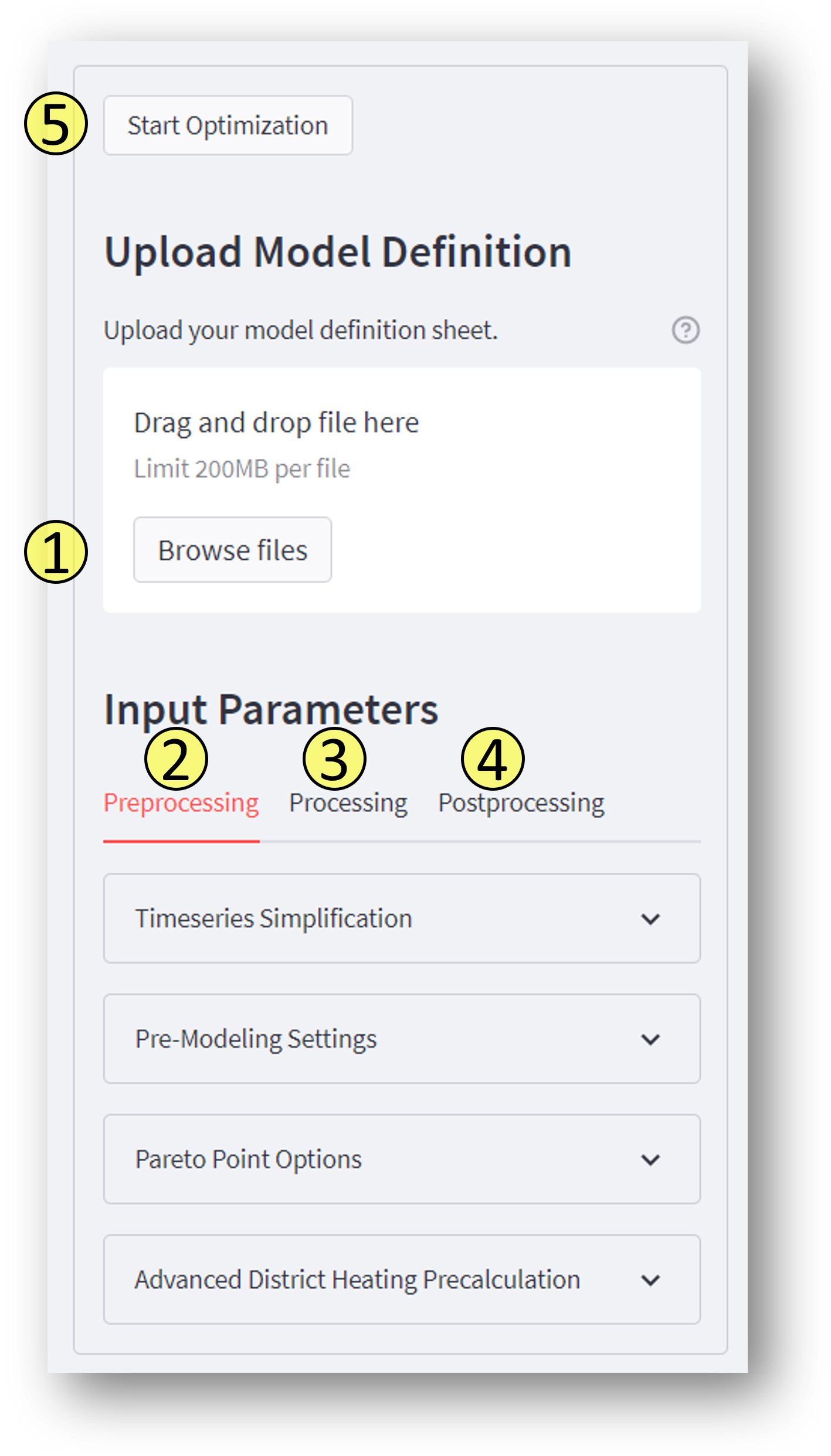
1. Adding the model definition
Here you can upload your model_definition.xlsx. After the file has been uploaded, you can theoretically continue with step 5. However, it is useful to make settings to reduce the computing time, since only limited computing resources are available.
2. Preprocessing
There are several ways to simplify the model. The method can be found here: Modeling Method. In the following, only the application is briefly described.
Timeseries Simplificaton
Warning
All time series simplifications can currently only be applied at an input time resolution of hours with 8760 time steps (i.e. one whole year). The algorithm described in the following sub-sections can be applied. Depending on the simplification applied, further adjustments to the energy system area automatically carried out.
Depending on which of the time series preparation algorithms described in the methods section is used, the following specifications must be made:
Algorithm: Indication of the simplification algorithm to be applied.
Index: Algorithm specific configuration.
Criterion: Criterion according to which cluster algorithms are applied.
Period: Time periods which are clustered together (weeks, days, hours)
Season: Time periods within which clustering takes place (year, seasons, months)
The following algorithms are applicable and must be specified with the following additional information. A detailed description of the algorithms can be found in the methods section.
algorithm |
description |
index |
criterion |
period |
season |
|---|---|---|---|---|---|
k_means |
The k-means algorithm clusters the time periods (see period) in such a way; that the squared deviation of the cluster centers is minimal. From the time periods of one cluster the mean is calculated and returned as reference period of the cluster. For the decision the vector of a single parameter (see criterion) over the period duration is considered. |
number of clusters to be considered. The number of clusters equals the number of returned reference days. |
Clustering criterion to be considered (temperature; dhi; heat demand; electricity demand) |
Period length to be clustered (hours; days; or weeks) |
– |
averaging |
successive time periods (e.g. two consecutive days) are averaged and combined into one segment. |
number of periods to be averaged |
– |
length of periods to be averaged (hours; days; weeks) |
– |
slicing A |
every n-th period is selected and considered within the modeling |
index = n (every n-th period is selected in the modeling) |
– |
length of periods to be sliced (hours; days; weeks) |
– |
slicing B |
every n-th period is deleted and removed from the modeling |
index = n (every n-th period is removed) |
– |
length of periods to be sliced (hours; days; weeks) |
– |
downsampling A |
Adaption of the temporal resolution. Every n-th period (selected by index column) is used for the modeling. For example; the resolution can be changed from a 1-hourly to a 3-hourly (index = 3) temporal resolution [1]. |
index = n (setting the new resolution) |
– |
– |
– |
downsampling B |
Adaption of the temporal resolution. Every n-th period (selected by index column) is deleted for the modeling. |
index = n (determination of the time steps to be deleted) |
– |
– |
– |
heuristic selection |
representative time periods of a time series are selected from certain selection criteria |
applied selection scheme (available schemes are listed here |
– |
length of periods to be selected (days or weeks) |
– |
random sampling |
a given number of random periods are selected and used as representatives |
number of periods to be selected. |
– |
length of periods to be selected randomly (days or weeks |
– |
Pre-Modeling Settings
Activate Pre-Modeling: If activated, the modeling process is divided into a pre-model and a main-model run.
Investment Boundaries Tightening: Must be checked, if the investment boundaries in the main-model shall be tightened based on the pre-model results.
Investment Tightening Factor: All investment limits of the main-model are limited to the investment decisions made in the pre-model run multiplied by this factor. If a originally defined investment boundary is lower than this value, the limit will not be changed.
Time Series Simplification: Timeseries simplification for the pre-model have to be set (see above for detailed description).
Pareto Point Options
Choose pareto point(s) if you want to start an pareto optimization run. The chosen value defines the constraint reduction in percent referring to the cost minimal pareto point. The values are given in percent.
Advances District Heating Precalculation
Clustering District Heating Network: The function allows to group the consumers of a street section into a clustered consumer when optimizing the heat network. This consumer is positioned at the averaged location.
Activate District Heating Precalculations: With use of this function it is possible to use the result folder of a model definition after the first optimization to skip the perpendicular foot print search by using the already existing calculations (this is usually quite time-consuming). For this purpose, the result folder must be specified in the drop-down menu below.
Switch Criteria
If you activate this field, you set instead of the primary costs (e. g. monetary costs), the constraining costs (e. g. GHG-Emissions) as the optimization variable, so you perform an e. g. emission-optimized run. The field is intended for single-criteria optimization only. In case of multi-criteria optimization, the optimization criteria will be changed automatically.
3. Processing
Number of threads: Number of threads to use for the model run on your machine. You should make sure that the chosen solver supports enough threats (cbc: max. 1 (if no parallelized version), gurobi: max. 8).
Optimization Solver: Chose on of the supported solver. Make sure that the solver is configurated on your machine. We recommend using the gurobi solver if you can use an academic licence.
4. Postprocessing
Create xlsx-files: Must be checked, if you want to get result files of every bus. The field should only be checked if users have in-depth model knowledge.
5. Starting the optimization
The button starts the optimization. After the optimization process you will be automatically redirected to the Result Processing page.
Model Definition
For the modeling and optimization of an energy system, parameters for all system components must be given in the model generator using the enclosed .xlsx file (editable with Excel, LibreOffice, …). The .xlsx file is divided into nine input sheets. In the “energysystem” sheet, general parameters are defined for the time horizon to be examined, in the sheets “buses”, “sinks”, “sources”, “transformers”, “storages” and “links” corresponding components are defined. In the sheet “time series”, the performance of individual components can be stored. In the “weather data” sheet, the required weather data is stored. When completing the input file, it is recommended to enter the energy system step by step and to perform test runs in between, so that potential input errors are detected early and can be localized more easily. In addition to the explanation of the individual input sheets, an example energy system is built step by step in the following subchapters. The input file for this example is stored in the program folder “examples” and viewed on GitHub. The following units are used throughout:
capacity/performance in kW,
energy in kWh,
angles in degrees, and
costs in cost units (CU).
Cost units are any scalable quantity used to optimize the energy system, such as euros or grams of carbon dioxide emissions.
Energysystem
Within this sheet, the time horizon and the temporal resolution of the model is defined. The following parameters have to be entered:
start date: Start of the modeling time horizon. Format: “YYYY-MM-DD hh:mm:ss”;
end date: End date of the modeling time horizon. Format: “YYYY-MM-DD hh:mm:ss”; and
temporal resolution: For the modelling considered temporal resolution. Possible inputs: “a” (years), “d” (days), “h” (hours), “min” (minutes), “s” (seconds), “ms” (milliseconds). Attention: Make sure to write in lower case letters.
timezone: By specifying the timezone, energy systems with correct time series (e.g. relevant for the correct balancing of the PV yield) can be modeled anywhere in the world. For this purpose, the pandas timezone string (e.g. Europe/Berlin) is inserted into the column. Then the start and end date, weather data and timeseries data which can be corrected to the UTC form for calculation.
periods: Number of periods within the time horizon (one year with hourly resolution equals 8760 periods). Attention: Number of periods has to equal length of Time series sheet and Weather data sheet.
cost limit in (CU): Value in order to set a limit for the whole energysystem, e.g. monetary costs. Set this field to “None” in order to ignore the limit. If you want to set a limit, you have to set specific values for each components seen below.
constraint cost limit in (CU): Value in order to set a limit for the whole energysystem, e.g. carbon dioxide emissions. Set this field to “None” in order to ignore the limit. If you want to set a limit, you have to set specific values for each components seen below.
minimum final energy reduction in (kWh): This value can be used to define how much final energy reduction must be achieved. Thus, the optimization algorithm is forced to save at least <your_value_here> kWh of final energy amount. Currently only insulation investments can be used to achieve reductions. The “constraint2” factor of the insulation measures is 1, since every kWh saved by insulation measures is fully included in the savings. This value is set in the algorithm and can currently not be changed by the user.
weather data lat: Latitude (WGS84) of the area under investigation. This value is used to import weather data from Open Energy Platform using feedinlib’s OpenFred.
weather data lon: Longitude (WGS84) of the area under investigation. This value is used to import weather data from Open Energy Platform using feedinlib’s OpenFred.
start date |
end date |
timezone |
temporal resolution |
periods |
cost limit |
constraint cost limit |
minimum final energy reduction |
weather data lat |
weather data lon |
|---|---|---|---|---|---|---|---|---|---|
(CU) |
(CU) |
||||||||
2012-01-01 00:00:00 |
2012-12-30 23:00:00 |
Europe/Berlin |
h |
8760 |
None |
None |
None |
None |
None |
Competition Constraints
The spreadsheet “Competition Constraints” allows you to match two or more components against a predefined limit. For example, an area competition. If you do not want to use this spreadsheet, it simply remains empty. To use this spreadsheet, the following values must be filled in:
label: Unique designation of the competition constraint. Also for competition constraints that are not activated.
comment: Space for an individual comment.
active: Specifies whether the competition constraint shall be included to the model. “0” = inactive, “1” = active.
component <number>: Label of the component that lays claim to the parameter which size set as the limit. Attention: <number> must be filled with consecutive integers (1, 2, 3…) for each row.
factor <number>: Factor that defines how many units of the target unit component <number> needs to provide 1 kW of power. Attention: <number> must be filled with consecutive integers (1, 2, 3…) for each row.
limit: Maximum size suitable for providing power (e.g. roof area for providing electricity and heat).
label |
comment |
active |
component 1 |
factor 1 |
component 2 |
factor 2 |
component 3 |
factor 3 |
limit |
|---|---|---|---|---|---|---|---|---|---|
unit/kW |
unit/kW |
unit/kW |
unit |
||||||
ID_competition |
1 |
ID_photovoltaic_electricity_source |
5.26 |
ID_solar_thermal_source |
1.79 |
None |
0 |
168 |
|
ID_three_component_competition |
0 |
ID_photovoltaic_electricity_source |
5.26 |
ID_solar_thermal_source |
1.79 |
ID_photovoltaic_source_changed_azimuth |
5.26 |
168 |
Buses
Within this sheet, the buses of the energy system are defined. The following parameters need to be entered:
label: Unique designation of the bus. Also for buses that are not activated. The following format is recommended: “<ID>_<energy sector>_bus”. <ID> and <energy sector> need to be replaced by the bus attributes.
comment: Space for an individual comment, e.g. an indication of which measure this component belongs to.
active: Specifies whether the bus shall be included to the model. “0” = inactive, “1” = active.
excess: Specifies whether to generate an excess sink, which consumes excess energy. “0” = no excess sink will be generated; “1” = excess sink will be generated.
shortage: Specifies whether to generate a shortage source that can compensate energy deficits or not. “0” = no shortage source will be generated; “1” = shortage source will be generated.
excess costs in (CU/kWh): Assigns a price per kWh to the release of energy to the excess sink. This can be specified either as a fixed price or as a time-dependent price series. If a price series is used, “timeseries” must be entered and must be provided in the Time series sheet. If the excess sink was deactivated, the fill character “0” is used.
shortage costs in (CU/kWh): Assigns a price per kWh to the purchase of energy from the shortage source. This can be specified either as a fixed price or as a time-dependent price series. If a price series is used, “timeseries” must be entered and must be provided in the Time series sheet. If the shortage source was deactivated, the fill character “0” is used.
excess constraint costs in (CU/kWh): Assigns a price per kWh to the release of energy to the excess sink referring to the constraint limit set in the Energysystem sheet. If the excess sink was deactivated or constraints are not considered, the fill character “0” is used.
shortage constraint costs in (CU/kWh): Assigns a price per kWh to the purchase of energy from the shortage source referring to the constraint limit set in the Energysystem sheet. If the shortage source was deactivated or constraints are not considered, the fill character “0” is used.
district heating conn. (exergy): This column allows you to specify whether the bus should be connected to the exergy heating network. If not, select “0”. If yes, either the nearest point of the heating network can be used as a connection (in this case the column must be filled with “dh-system” for inserting heat buses and with “1” for exporting heat busses), or one of the street points from the District Heating Sheet is used (in this case the column must be filled according to the following pattern: <label of the pipe part from District Heating Sheet>-1 for the first node or <label of the pipe part from District Heating Sheet>-2 for the second).
lat: This column must be filled if the bus should be connected to the network by the search of his nearest point (possible entries in district heating conn. (exergy) “dh-system” or “1”). It has to be filled with the buses latitude (WGS84).
lon: This column must be filled if the bus should be connected to the network by the search of his nearest point (possible entries in district heating conn. (exergy) “dh-system” or “1”). It has to be filled with the buses longitude (WGS84).
existing heathouse station: Specifies whether costs are incurred for the use of a heathouse station, which is necessary for the connection of the exporting bus to the exergy heating network.
district heating conn. (anergy): This column allows you to specify whether the bus should be connected to the anergy heating network. If not, select “0”. If yes, either the nearest point of the heating network can be used as a connection (in this case the column must be filled with “dh-system” for inserting heat buses and with “1” for exporting heat busses), or one of the street points from the District Heating Sheet is used (in this case the column must be filled according to the following pattern: <label of the pipe part from District Heating Sheet>-1 for the first node or <label of the pipe part from District Heating Sheet>-2 for the second).
flow temperature in (°C): As the calculation of the coefficient of performance (COP) of the anergy heat pump which is required to connect the exporting buses to the anergy network, requires a temperature difference, the operating temperature level of the heat bus to be connected must be specified here.
electricity bus: As the anergy heat pump requires an amount of electricity during operation, the label of the electricity bus supplying it must be specified here.
sector: This column is used to assign the shortages of the buses to the energy amount diagrams in the result processing. Possible entries: electricity, heat, cooling, central_electricity, central_heat, central_cooling and None for buses that cannot be assigned to any category.
label |
comment |
active |
excess |
shortage |
excess costs |
shortage costs |
excess constraint costs |
shortage constraint costs |
district heating conn. (exergy) |
lat |
lon |
existing heathouse station |
district heating conn. (anergy) |
flow temperature |
electricity bus |
sector |
|---|---|---|---|---|---|---|---|---|---|---|---|---|---|---|---|---|
(CU/kWh) |
(CU/kWh) |
(CU/kWh) |
(CU/kWh) |
(°C) |
||||||||||||
ID_electricity_bus |
1 |
0 |
1 |
0.000 |
0.300 |
0.000 |
474.000 |
0 |
0 |
0 |
0 |
0 |
0 |
0 |
electricity |
|
ID_heat_bus |
1 |
0 |
0 |
0.000 |
0.000 |
0.000 |
0.000 |
0 |
50.05 |
7.05 |
0 |
0 |
0 |
0 |
heat |
|
ID_gas_bus |
1 |
0 |
1 |
0.000 |
0.070 |
0.000 |
0.000 |
0 |
0 |
0 |
0 |
0 |
0 |
0 |
None |
|
ID_cooling_bus |
1 |
0 |
0 |
0.000 |
0.000 |
0.000 |
0.000 |
0 |
0 |
0 |
0 |
0 |
0 |
0 |
cooling |
|
ID_pv_bus |
1 |
1 |
0 |
-0.068 |
0.000 |
-56.000 |
0.000 |
0 |
0 |
0 |
0 |
0 |
0 |
0 |
electricity |
|
ID_hp_electricity_bus |
1 |
0 |
1 |
0.000 |
0.220 |
0.000 |
474.000 |
0 |
0 |
0 |
0 |
0 |
0 |
0 |
electricity |
|
district_electricity_bus |
0 |
0 |
0 |
0.000 |
0.000 |
0.000 |
0.000 |
0 |
0 |
0 |
0 |
0 |
0 |
0 |
central_electricity |
|
district_heat_bus |
0 |
0 |
0 |
0.000 |
0.000 |
0.000 |
0.000 |
dh-system |
50.00 |
10.00 |
0 |
0 |
0 |
0 |
central_heat |
|
district_chp_electricity_bus |
0 |
0 |
1 |
-0.068 |
0.000 |
-375.00 |
0.000 |
0 |
0 |
0 |
0 |
0 |
0 |
0 |
central_electricity |
|
district_gas_bus |
0 |
0 |
1 |
0.000 |
0.070 |
0.000 |
0.000 |
0 |
0 |
0 |
0 |
0 |
0 |
0 |
None |
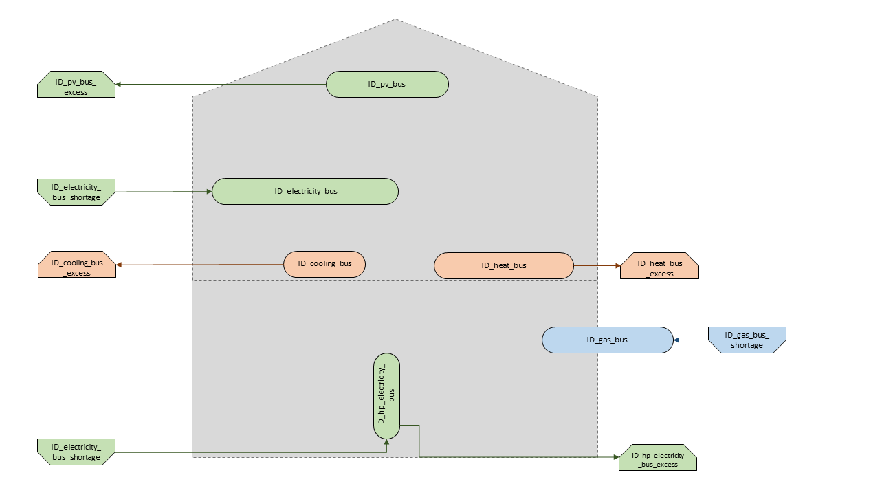
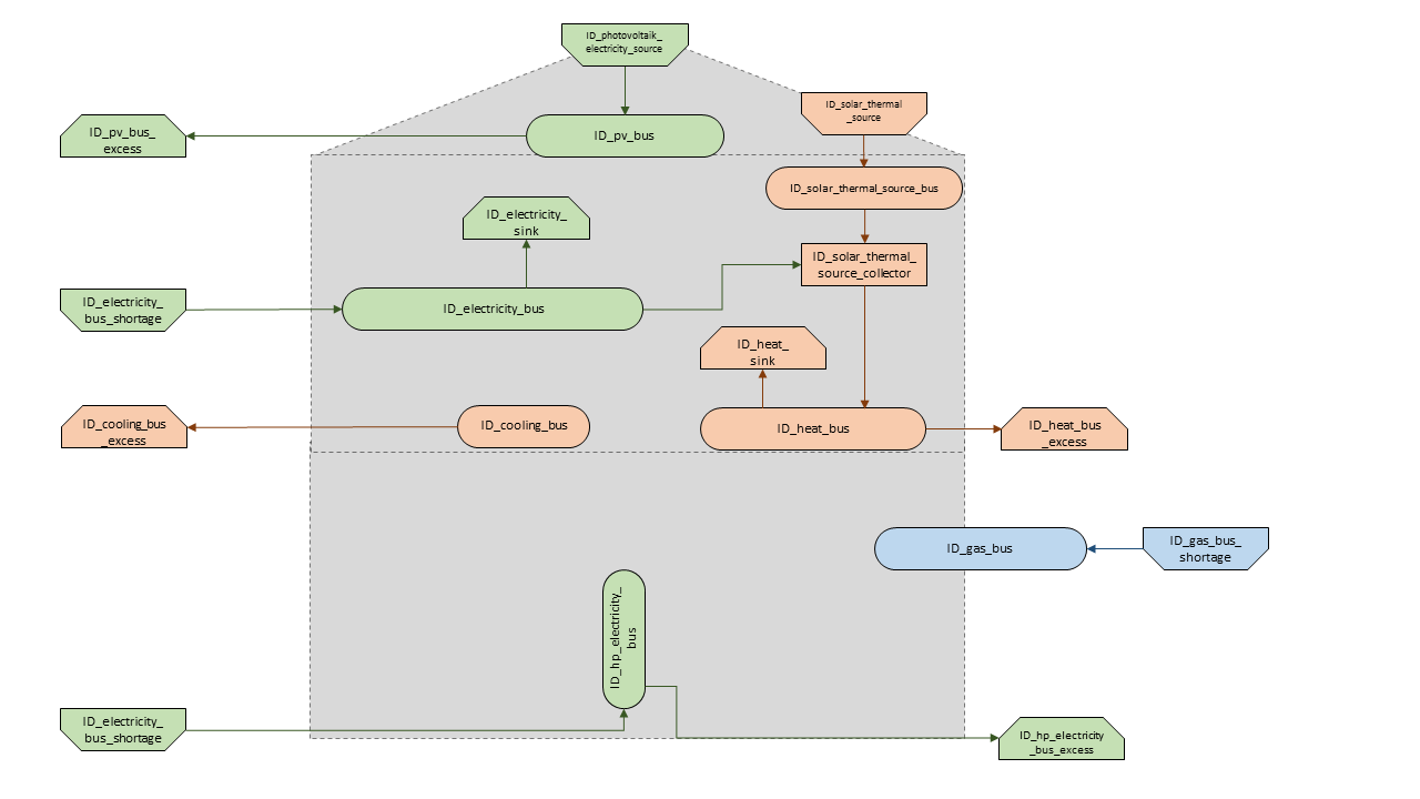
Graph of the energy system, which is created by entering the example components. The non-active components are not included in the graph above.
District Heating
Within this sheet, the road network structure of the energy system is defined. The following parameters need to be entered:
label: Unique designation of the street section, e.g. the street section name. Also for streets that are not activated.
comment: Space for an individual comment.
active: Specifies whether the street section shall be included to the model. “0” = inactive, “1” = active.
lat. 1st intersection: Latitude (WGS84) of the first point of the given street part.
lon. 1st intersection: Longitude (WGS84) of the first point of the given street part.
lat. 2nd intersection: Latitude (WGS84) of the second point of the given street part.
lon. 2nd intersection: Longitude (WGS84) of the second point of the given street part.
label |
comment |
active |
lat. 1st intersection |
lat. 2nd intersection |
lat. 1st intersection |
lon. 2nd intersection |
|---|---|---|---|---|---|---|
ID_street1 |
1 |
45.00 |
55.00 |
5.00 |
10.00 |
Sinks
Within this sheet, the sinks of the energy system are defined. The following parameters need to be entered:
label: Unique designation of the sink. Also for sinks that are not activated. The following format is recommended: “<ID>_<energy sector>_sink”. <ID> and <energy sector> need to be replaced by the sink attributes.
comment: Space for an individual comment, e.g. an indication of which measure this component belongs to.
active: Specifies whether the sink shall be included to the model. “0” = inactive, “1” = active.
fixed: Specifies whether it is a fixed sink or not. “0” = not fixed; “1” = fixed.
input: Specifies the bus from which the input to the sink comes from.
load profile: Specifies the basis onto which the load profile of the sink is to be created. If the Richardson tool is to be used, “richardson” has to be inserted. For standard load profiles, its acronym is used. The different load profiles are explained here. If a time series is used, “timeseries” must be entered and must be provided in the Time series sheet. If the sink is not fixed, the fill character “x” has to be used.
nominal value in (kW): Nominal performance of the sink. Required when “timeseries” has been entered into the “load profile”. When SLP or Richardson is used, use the fill character “0” here.
annual demand in (kWh/a): Annual energy demand of the sink. Required when using the Richardson Tool or standard load profiles. When using time series, the fill character “0” is used.
occupants [RICHARDSON]: Number of occupants living in the respective building. Only required when using the Richardson tool, use fill character “0” for other load profiles.
building class [HEAT SLP ONLY]: The BDEW building classes are needed for the creating of the non-commercial slp. The parameter building_class (German: Baualtersklasse) can assume values in the range 1-11. The different building classes are explained here (building class 12 was added later and is therefore not available). For non-residential buildings the building class “0” is used.
wind class [HEAT SLP ONLY]: Wind classification for building location (“0” = not windy, “1” = windy).
sector: This column is used to assign the sinks’ energy amounts to the energy amount diagrams in the result processing. Possible entries: electricity, heat, cooling.
label |
comment |
active |
fixed |
input |
load profile |
nominal value |
annual demand |
occupants |
building class |
wind class |
sector |
|---|---|---|---|---|---|---|---|---|---|---|---|
(kW) |
(kWh/a) |
(richardson) |
(heat slp) |
(heat slp) |
|||||||
ID_electricity_sink |
1 |
1 |
ID_electricity_bus |
h0 |
0 |
5000.0 |
0 |
0 |
0 |
electricity |
|
ID_heat_sink |
1 |
1 |
ID_heat_bus |
efh |
0 |
30000.0 |
0 |
3 |
0 |
heat |
|
ID_cooling_sink |
0 |
1 |
ID_cooling_bus |
timeseries |
1 |
0 |
0 |
0 |
0 |
cooling |
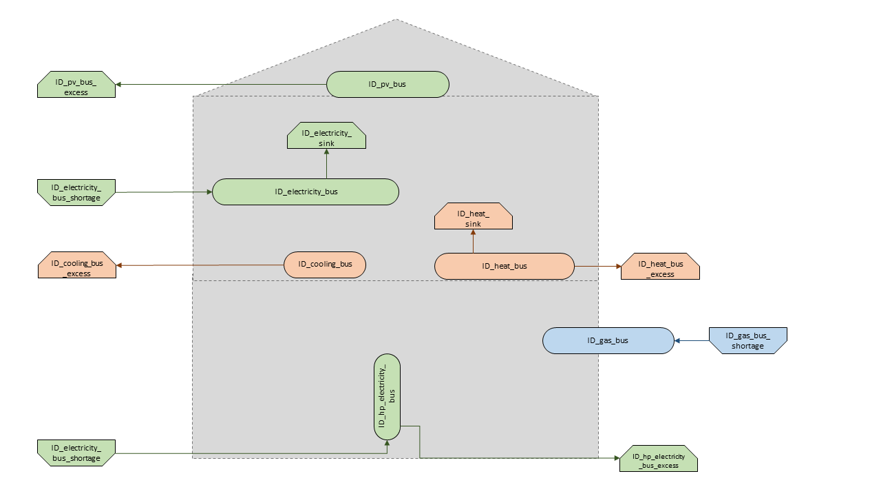
Graph of the energy system, which is created by entering the example components. The non-active components are not included in the graph above.
Sources
Within this sheet, the sources of the energy system are defined. Technology specific data (see 2nd line), must be filled in only if the respective technology is selected otherwise use “0”. The following parameters have to be entered:
label: Unique designation of the source. Also for sources that are not activated. The following format is recommended: “<ID>_<energy sector>_source”. <ID> and <energy sector> need to be replaced by the bus attributes.
comment: Space for an individual comment, e.g. an indication of which measure this component belongs to.
active: Specifies whether the source shall be included to the model. “0” = inactive, “1” = active.
fixed: Indicates whether it is a fixed source or not. “0” = not fixed; “1” = fixed.
output: Specifies which bus the output of the source is connected to.
input: Specifies which bus the input of the source is connected to (currently not required for any technology).
technology: Technology type of source. Input options: “photovoltaic”, “windpower”, “timeseries”, “other”, “solar_thermal_flat_plate”, “concentrated_solar_power”. Time series are automatically generated for photovoltaic systems and wind turbines. If “timeseries” is selected, a time series must be provided in the Time series sheet.
sector: This column is used to differentiate between an electricity, heat and cooling source for the result processing energy amount collection. Possible entries: “electricity”, “heat”, “cooling”, “central_electricity”, “central_heat”, “central_cooling”.
Costs
existing capacity in (kW): Existing capacity of the source before possible investment.
min. investment capacity in (kW): Minimum capacity to be installed in case of an investment.
max. investment capacity in (kW): Maximum capacity that can be added in the case of an investment. If no investment is possible, enter the value “0” here.
variable costs in (CU/kWh): Defines the variable costs incurred for a kWh of energy drawn from the source.
variable constraint costs in (CU/kWh): Defines the variable costs incurred for a kWh of energy drawn from the source referring to the constraint limit set in the “energysystem” sheet. If not considering constraints fill character “0” is used.
periodical costs in (CU/(kW a)): Costs incurred per kW for investments within the time horizon. Periodical costs only apply for newly invested capacities but not for existing capacities.
periodical constraint costs in (CU/(kW a)): Costs incurred per kW for investments within the time horizon referring to the constraint limit set in the “energysystem” sheet. If not considering constraints fill character “0” is used.
non-convex investment: Specifies whether the investment capacity should be defined as a mixed-integer variable, i.e. whether the model can decide whether NOTHING OR THE INVESTMENT should be implemented. Explained here.
fix investment costs in (CU/a): Fixed costs of non-convex investments (in addition to the periodic costs).
fix investment constraint costs in (CU/a): Fixed constraint costs of non-convex investments (in addition to the periodic constraint costs).
Wind
The following parameters need to be set for wind power sources.
The wind speed timeseries entered in the Weather data sheet (measured at 10 m height) will get converted into wind speeds at specified hub height. With the specified turbine model an energy timeseries will then be calculated.
Turbine Model: Reference wind turbine model. Possible turbine types are listed in the windpowerlib’s database. Write the value of the column “turbine_type” of the .csv in your spreadsheet.
Hub Height: Hub height of the wind turbine. Which hub heights are possible for the selected reference turbine can be viewed in the windpowerlib’s database too.
PV
The parameters for PV sources depend on the selected technology.
General PV Parameters
Azimuth: Specifies the orientation of the PV module in degrees. Values between “0” and “360” are permissible (“0” = north, “90” = east, “180” = south, “270” = west). Use fill character “0” for other technologies.
Surface Tilt: Specifies the inclination of the module in degrees (“0” = flat). Use fill character “0” for other technologies.
Albedo: Specifies the albedo value of the reflecting floor surface. Only required for photovoltaic sources, use fill character “0” for other technologies.
Altitude: Height (above mean sea level) in meters of the photovoltaic module. Only required for photovoltaic sources, use fill character “0” for other technologies.
Latitude: Geographic latitude (decimal number in WGS84) of the photovoltaic module. Only required for photovoltaic sources, use fill character “0” for other technologies.
Longitude: Geographic longitude (decimal number in WGS84) of the photovoltaic module. Only required for photovoltaic sources, use fill character “0” for other technologies.
DC AC ratio: Defines the ratio of the DC module capacity to the inverter’s AC rated capacity ($P_{DC} / P_{AC}$). This value is mandatory for all PV configurations to correctly scale the inverter limits. Example: A value of 1.2 means the DC plant capacity is 20% larger than the inverter’s maximum AC output. If you want no undersizing/clipping at all, use 1.0. Only required for photovoltaic sources, use fill character “0” for other technologies.
Module Definition
Depending on your technology choice, define the module via database OR manual datasheet entry:
Option A: Database lookup
Modul Model: Module name, according to the database used (see PVLIB database Sandia or PVLIB database CEC ). Possible Modul Models are presented here. Use fill character “0” for other technologies.
Option B: Manual datasheet
Power STC: Power at Standard Test Conditions (STC) in Watt (e.g. 235). Use fill character “0” for other technologies.
Celltype: Type of the solar cell. Possible entries: “monoSi”, “multiSi”, “polySi”, “cis”, “cigs”, “cdte”, “amorphous”. Use fill character “0” for other technologies.
V mp: Voltage at maximum power point in Volt (e.g. 43). Use fill character “0” for other technologies.
I mp: Current at maximum power point in Ampere (e.g. 5,48). Use fill character “0” for other technologies.
V oc: Open-circuit voltage in Volt (e.g. 51,8). Use fill character “0” for other technologies.
I sc: Short-circuit current in Ampere (e.g. 5,84). Use fill character “0” for other technologies.
Alpha sc: Temperature coefficient of the short-circuit current in A/°C (e.g. 0,00175). Data sheets often specify this in %/°C; it must be converted to an absolute value by dividing the percentage by 100 and multiplying the result by the short-circuit current (i_sc). Use fill character “0” for other technologies.
Beta voc: Temperature coefficient of the open-circuit voltage in V/°C (e.g. -0,124). Data sheets often specify this in %/°C; it must be converted to an absolute value by dividing the percentage by 100 and multiplying the result by the open-circuit voltage (v_oc). Use fill character “0” for other technologies.
Gamma pmp: Temperature coefficient of the maximum power point power in %/°C (e.g., “-0.3”). This value is entered directly as a percentage. Use fill character “0” for other technologies.
Cells in series: Number of solar cells connected in series within one module (e.g. 72). Use fill character “0” for other technologies.
Inverter Definition
Define how the inverter is modeled. This works independently of the chosen module technology:
Option A: Database lookup
Inverter Model: Inverter name, according to the database used. Possible Inverter Models are presented here. If found in the database, only the efficiency characteristics (the efficiency curve) of the inverter are used for the simulation. To prevent artificial clipping or unintended shutdowns in single-module simulations, all lower operational thresholds, such as the startup power threshold ($P_{so}$) or minimum MPPT voltage, are programmatically disabled (set to 0). Meanwhile, the inverter’s capacity limits are programmatically normalized and scaled using the mandatory dc_ac_ratio to match the DC system size. Use fill character “0” for other technologies or if you want to use a constant efficiency instead.
Option B: Constant efficiency fallback
Inverter eta: Nominal inverter efficiency as a decimal fraction (e.g., 0.96 for 96% efficiency). This parameter acts as a fallback and is only evaluated if the specified “Inverter Model” is not found in any database. If used, the system falls back to a simplified PVWatts inverter model. Use fill character “0” for other technologies.
Concentrated Solar Power
The following parameters need to be set for concentrated solar power sources.
Azimuth: Specifies the orientation of the PV module in degrees. Values between “0” and “360” are permissible (“0” = north, “90” = east, “180” = south, “270” = west). Use fill character “0” for other technologies.
Surface Tilt: Specifies the inclination of the module in degrees (“0” = flat). Use fill character “0” for other technologies.
ETA 0: Optical efficiency of the collector. Use fill character “0” for other technologies.
A1 in (1/°): Collector specific linear heat loss coefficient. Use fill character “0” for other technologies.
A2 in (1/°)2: Collector specific quadratic heat loss coefficient. Use fill character “0” for other technologies.
C1 in (W/m2 K): Collector specific thermal loss parameter. Only required for concentrated solar power source, use fill character “0” for other technologies.
C2 in (W/m2 K2): Collector specific thermal loss parameter. Only required for concentrated solar power source, use fill character “0” for other technologies.
Temperature Inlet in (°C): Inlet temperature of the solar heat collector module. Use fill character “0” for other technologies.
Temperature Difference in (°C): Temperature Difference between mean and inlet temperature of the solar heat collector module. Use fill character “0” for other technologies.
Cleanliness: Cleanliness of a parabolic through collector. Only required for Concentrated Solar Power source, use fill character “0” for other technologies.
Peripheral Losses: Heat loss coefficient for losses in the collector’s peripheral system. Use fill character “0” for other technologies.
Exemplary values for concentrated_solar_power technology:
Cleanliness |
ETA 0 |
A1 |
A2 |
C1 |
C2 |
|---|---|---|---|---|---|
solar heat |
solar heat |
solar heat |
solar heat |
solar heat |
solar heat |
0.9 |
0.816 |
-0.00159 |
0.0000977 |
0.0622 |
0.00023 |
Solar Thermal Flat Plate
The following parameters need to be set for solar thermal flat plate sources.
Azimuth: Specifies the orientation of the PV module in degrees. Values between “0” and “360” are permissible (“0” = north, “90” = east, “180” = south, “270” = west). Use fill character “0” for other technologies.
Surface Tilt: Specifies the inclination of the module in degrees (“0” = flat). Use fill character “0” for other technologies.
ETA 0: Optical efficiency of the collector. Use fill character “0” for other technologies.
A1 in (1/°): Collector specific linear heat loss coefficient. Use fill character “0” for other technologies.
A2 in (1/°)2: Collector specific quadratic heat loss coefficient. Use fill character “0” for other technologies.
Temperature Inlet in (°C): Inlet temperature of the solar heat collector module. Use fill character “0” for other technologies.
Temperature Difference in (°C): Temperature Difference between mean and inlet temperature of the solar heat collector module. Use fill character “0” for other technologies.
Peripheral Losses: Heat loss coefficient for losses in the collector’s peripheral system. Use fill character “0” for other technologies.
Conversion Factor in (m2 /kW): The factor is explained here.
Timeseries
If you have chosen the technology “timeseries” (in the technology column), you have to include a timeseries in the Time series sheet or use default one.
Commodity
If you have chosen the technology “other” (in the technology column), a commodity source with maximum investable capacity but completely variable time series becomes part of the energy system. The solver can thus design a completely linear source and use it to cover the demand when required.
label |
comment |
active |
fixed |
technology |
output |
input |
existing capacity |
min. investment capacity |
max. investment capapcity |
non-convex investment |
fix investment costs |
variable costs |
periodical costs |
variable constraint costs |
periodical constraint costs |
Turbine Model |
Hub Height |
Modul Model |
Inverter Model |
DC AC Ratio |
Inverter Eta |
Albedo |
Altitude |
Azimuth |
Surface Tilt |
Latitude |
Longitude |
ETA 0 |
A1 |
A2 |
C1 |
C2 |
Temperature Inlet |
Temperature Difference |
Conversion Factor |
Peripheral Losses |
Cleanliness |
power stc |
celltype |
v mp |
i mp |
v oc |
i sc |
alpha sc |
beta voc |
gamma pmp |
cells in series |
sector |
|
|---|---|---|---|---|---|---|---|---|---|---|---|---|---|---|---|---|---|---|---|---|---|---|---|---|---|---|---|---|---|---|---|---|---|---|---|---|---|---|---|---|---|---|---|---|---|---|---|---|---|
solar heat |
(kW) |
(kW) |
(kW) |
(CU/a) |
(CU/kWh) |
(CU/(kW a)) |
(CU/kWh) |
(CU/(kW a)) |
windpower |
windpower |
PV |
PV |
PV |
PV |
PV |
(m) | PV |
(°) |
(°) |
(°) |
(°) |
solar heat |
(1/°) | solar heat |
(1/°)2 | solar heat |
(W/m2 K) | solar heat |
(W/m2 K2) | solar heat |
(°C) | solar heat |
(°C) | solar heat |
(m2/kW) | solar heat |
solar heat |
solar heat |
solar heat |
(W) | PV |
PV |
(V) | PV |
(A) | PV |
(V) | PV |
(A) | PV |
(A/°C) | PV |
(V/°C) | PV |
(%/°C) | PV |
PV |
||||||||
ID_photovoltaic_electricity_source |
1 |
1 |
photovoltaic |
ID_pv_bus |
None |
0 |
0 |
20 |
0 |
0 |
0 |
90 |
56 |
0 |
0 |
0 |
Panasonic_VBHN235SA06B__2013_ |
ABB__MICRO_0_25_I_OUTD_US_240__240V_ |
1 |
0 |
0.18 |
60 |
180 |
35 |
52.13 |
7.36 |
0 |
0 |
0 |
0 |
0 |
0 |
0 |
0 |
0 |
0 |
0 |
0 |
0 |
0 |
0 |
0 |
0 |
0 |
0 |
0 |
electricity |
||
ID_solar_thermal_source |
1 |
1 |
solar_thermal_flat_plate |
ID_heat_bus |
ID_electricity_bus |
0 |
0 |
20 |
0 |
0 |
0 |
40 |
25 |
0 |
0 |
0 |
0 |
0 |
0 |
0 |
0 |
0 |
20 |
10 |
52.13 |
7.36 |
0.719 |
1.063 |
0.005 |
0 |
0 |
40 |
15 |
1.79 |
0.05 |
0 |
0 |
0 |
0 |
0 |
0 |
0 |
0 |
0 |
0 |
0 |
heat |
||
wind_turbine |
0 |
1 |
windpower |
electricity_bus |
None |
0 |
0 |
30 |
0 |
0 |
0 |
100 |
9 |
0 |
E-126/4200 |
135 |
0 |
0 |
0 |
0 |
0 |
0 |
0 |
0 |
0 |
0 |
0 |
0 |
0 |
0 |
0 |
0 |
0 |
0 |
0 |
0 |
0 |
0 |
0 |
0 |
0 |
0 |
0 |
0 |
0 |
0 |
electricity |
||
ID_photovoltaic_electricity_source |
1 |
1 |
photovoltaic_datasheet |
ID_pv_bus |
None |
0 |
0 |
20 |
0 |
0 |
0 |
90 |
56 |
0 |
0 |
0 |
0 |
0 |
1 |
0.97 |
0.18 |
60 |
180 |
35 |
52.13 |
7.36 |
0 |
0 |
0 |
0 |
0 |
0 |
0 |
0 |
0 |
0 |
235 |
monoSi |
43 |
5.48 |
51.8 |
5.84 |
0.00175 |
-0.124 |
-0.3 |
72 |
electricity |
Graph of the energy system, which is created by entering the example components of sources sheet. The non-active components are not included in the graph above.
Transformers
Within this sheet, the transformers of the energy system are defined.
The following parameters have to be entered:
label: Unique designation of the transformer. Also for transformers that are not activated. The following format is recommended: “<ID>_<energy sector>_transformer”. <ID> and <energy sector> need to be replaced by the transformer attributes.
comment: Space for an individual comment, e.g. an indication of which measure this component belongs to.
active: Specifies whether the transformer shall be included to the model. “0” = inactive, “1” = active.
transformer type: Indicates what kind of transformer it is. Possible entries: “GenericTransformer” for linear transformers with constant efficiencies; “GenericTwoInputTransformer” for transformers with two inputs and constant efficiencies (e. g. Pumping units with water and electricity intake); “GenericCHP” for transformers with varying efficiencies; “CompressionHeatTransformer”; “AbsorptionHeatTransformer”.
mode: Specifies, if a compression or absorption heat transformer is working as “chiller” or “heat_pump”. Only required if “transformer type” is set to “CompressionHeatTransformer” or “AbsorptionHeatTransformer”. Otherwise has to be set to “0”.
input: Specifies the bus from which the input to the transformer comes from.
input2: Specifies the bus from which the secondary input of the transformer comes from. Only required if “transformer type” is set to “GenericTwoInputTransformer”. If there is no second input, the fill character “0” must be entered here.
output: Specifies bus to which the output of the transformer is forwarded to. If the sector “central_heat” is selected for a CHP the electrical output bus must be used here. If the sector “central_electricity” is selected for a CHP the heat output bus must be used here.
output2: Specifies the bus to which the secondary output of the transformer is forwarded to. If there is no second output, the fill character “0” must be entered here.
input2 / input: Specifies the ratio of input2 to input (e.g. kWh/m3). The ratio is further used to calculate to factors for the input flows. If a transformer uses two inputs of the same types with different amounts this can also be considered with the ratio (e.g. 60% biogas and 40% naturalgas can be translated to a ratio of 0,6/0,4=1,25). Only required if “transformer type” is set to “GenericTwoInputTransformer”. If there is no second input, the fill character “0” must be entered here.
sector: This column is used to differentiate the transformer types for the result processing energy amount collection. Possible entries: “electricity”, “heat”, “cooling”, “central_electricity”, “central_heat”, “central_cooling”, “electric_heating”.
technology: The technology column represents the category in which the energy quantities for the energy quantity diagrams are collected. If, for example, “natural_gasheating” is entered for a component, it will appear under natural_gasheating in the energy quantity diagram. Attention: If in the sector “central_”… is used in the sector, a leading “central_” is appended to the selected technology in the balancing.
Costs
existing capacity in (kW): Existing capacity of the transformer before possible investment.
min investment capacity in (kW): Minimum transformer capacity to be installed.
max investment capacity in (kW): Maximum installable transformer capacity regarding the output of the transformer, in addition to previously installed capacity, if existing.
variable input costs in (CU/kWh): Variable costs incurred per kWh of input energy supplied.
variable input costs 2 in (CU/kWh): Variable costs incurred per kWh of input 2 energy supplied.
variable output costs in (CU/kWh): Variable costs incurred per kWh of output energy supplied.
variable output costs 2 in (CU/kWh): Variable costs incurred per kWh of output 2 energy supplied.
variable input constraint costs in (CU/kWh): Variable constraint costs incurred per kWh of input energy supplied referring to the constraint limit set in the “energysystem” sheet. If not considering constraints fill character “0” is used.
variable input constraint costs 2 in (CU/kWh): Variable constraint costs incurred per kWh of input2 energy supplied referring to the constraint limit set in the “energysystem” sheet. If not considering constraints fill character “0” is used.
variable output constraint costs in (CU/kWh): Variable constraint costs incurred per kWh of output energy supplied referring to the constraint limit set in the “energysystem” sheet. If not considering constraints fill character “0” is used.
variable output constraint costs 2 in (CU/kWh): Variable constraint costs incurred per kWh of output 2 energy supplied referring to the constraint limit set in the “energysystem” sheet. If not considering constraints fill character “0” is used.
periodical costs in (CU/a): Costs incurred per kW for investments within the time horizon. Periodical costs only apply for newly invested capacities but not for existing capacities.
periodical constraint costs in (CU/(kW a)): Constraint costs incurred per kW for investments within the time horizon. If not considering constraints fill character “0” is used.
non-convex investment: Specifies whether the investment capacity should be defined as a mixed-integer variable, i.e. whether the model can decide whether NOTHING OR THE INVESTMENT should be implemented. Explained here.
fix investment costs in (CU/a): Fixed costs of non-convex investments (in addition to the periodic costs).
fix investment constraint costs in (CU/a): Fixed constraint costs of non-convex investments (in addition to the periodic constraint costs).
Generic Transformer
efficiency: Specifies the efficiency of the first output. Values between “0” and “1” are allowed entries.
efficiency2: Specifies the efficiency of the second output, if there is one. Values between “0” and “1” are entered. If there is no second output, the fill character “0” must be entered here.
Compression Heat Transformer
The following parameters are only required, if “transformer type” is set to “CompressionHeatTransformer”:
heat source: Specifies the heat source. Possible heat sources are “GroundWater”, “Ground”, “Air”, “Air-to-Air” (which represents an AAHP) and “Water”.
temperature high in (°C): Temperature of the high temperature heat reservoir. Only required if “mode” is set to “heat_pump”.
temperature low in (°C): Cooling temperature needed for cooling demand. Only required if “mode” is set to “chiller”.
quality grade: To determine the COP of a real machine a scale-down factor (the quality grade) is applied on the Carnot efficiency (see oemof.thermal).
area in (m2): Open spaces for ground-coupled compression heat transformers (GCHP).
length of the geoth. probe in (m): Length of the vertical heat exchanger, only for GCHP.
heat extraction in (kW/(m a)): Heat extraction for the heat exchanger referring to the location, only for GCHP.
min. borehole area in (m2): Limited space due to the regeneration of the ground source, only for GCHP.
temp threshold icing: Temperature below which icing occurs (see oemof.thermal). Only required if “mode” is set to “heat_pump”.
factor icing: Factor to which the COP is reduced caused by icing (e.g. “0.8” if you have a reduction of 20%) (see oemof.thermal). Only required if “mode” is set to “heat_pump”.
Absorption Heat Transformer
The following parameters are only required, if “transformer type” is set to “AbsorptionHeatTransformer”:
name: Defines the way of calculating the efficiency of the absorption heat transformer. Possible inputs are: “Rotartica”, “Safarik”, “Broad_01”, “Broad_02”, and “Kuehn”. “Broad_02” refers to a double-effect absorption chiller model, whereas the other keys refer to single-effect absorption chiller models.
temperature high in (°C): Temperature of the heat source, that drives the absorption heat transformer.
temperature low in (°C): Output temperature which is needed for the cooling demand.
electrical input conversion factor: Specifies the relation of electricity consumption to energy input. Example: A value of “0,05” means, that the system consumes 5 % of the input energy as electric energy.
recooling temperature difference in (°C): Defines the temperature difference between temperature source for recooling and recooling cycle.
heat capacity of source: Defines the heat capacity of the connected heat source e.g. extracted waste heat.
GenericCHP
Warning
Currently the GenericCHP component can only be used for the purpose of simulation. The solver is not able to dimension the components capacity. Since there is no investment decision no periodical costs apply.
min. share of flue gas loss: Percentage flue gas losses of the operating point with maximum heat extraction.
max. share of flue gas loss: Percentage flue gas losses of the operating point with minimum heat extraction.
min. electric power in (kW): Minimum electrical power supply without heat extraction (district heating).
max. electric power in (kW): Maximum electrical power supply without heat extraction (district heating).
min. electric efficiency: Specifies the minimum electric efficiency without heat extraction (district heating). Values between “0” and “1” are allowed entries.
max. electric efficiency: Specifies the minimum electric efficiency without heat extraction (district heating). Values between 0 and 1 are allowed entries.
minimal thermal output power in (kW): Heat output taken from the exhaust gas via a condenser even in purely electric operation.
electric power loss index: Reduction of the electrical power by “electric power loss index * extracted thermal power”.
back pressure: Defines rather the end pressure of “Turbine CHP” is higher than ambient pressure (input value has to be “1”) or not (input value has to be “0”). For “Motoric CHP” it has to be “0”.
label |
comment |
active |
transformer type |
mode |
input |
input2 |
output |
output2 |
input2 / input |
efficiency |
efficiency2 |
existing capacity |
min. investment capacity |
max. investment capacity |
non-convex investment |
fix investment costs |
variable input costs |
variable input costs 2 |
variable output costs |
variable output costs 2 |
periodical costs |
variable input constraint costs |
variable input constraint costs 2 |
variable output constraint costs |
variable output constraint costs 2 |
periodical constraint costs |
heat source |
temperature high |
temperature low |
quality grade |
area |
length of the geoth. probe |
heat extraction |
min. borehole area |
temp. threshold icing |
factor icing |
name |
electrical input conversion factor |
recooling temperature difference |
min. share of flue gas loss |
max. share of flue gas loss |
min. electric power |
max. electric power |
min. electric efficiency |
max. electric efficiency |
minimal thermal output power |
elec. power loss index |
back pressure |
sector |
technology |
|---|---|---|---|---|---|---|---|---|---|---|---|---|---|---|---|---|---|---|---|---|---|---|---|---|---|---|---|---|---|---|---|---|---|---|---|---|---|---|---|---|---|---|---|---|---|---|---|---|---|---|
(kW) |
(kW) |
(kW) |
(CU/a) |
(CU/kWh) |
(CU/kWh) |
(CU/kWh) |
(CU/kWh) |
(CU/(kW a)) |
(CU/kWh) |
(CU/kWh) |
(CU/kWh) |
(CU/kWh) |
(CU/(kW a)) |
(°C) |
(°C) |
(m2) |
(m) |
(kW/(m a)) |
(m2) |
(°C) |
(°C) |
(kW) |
(kW) |
(kW) |
||||||||||||||||||||||||||
ID_gasheating_transformer |
1 |
GenericTransformer |
0 |
ID_gas_bus |
0 |
ID_heat_bus |
0 |
0 |
0.85 |
0 |
0 |
0 |
20 |
0 |
0 |
0 |
0 |
0 |
0 |
70 |
0 |
0 |
200 |
0 |
0 |
0 |
0 |
0 |
0 |
0 |
0 |
0 |
0 |
0 |
0 |
0 |
0 |
0 |
0 |
0 |
0 |
0 |
0 |
0 |
0 |
0 |
0 |
heat |
natural_gasheating |
|
ID_TwoInput_transformer |
0 |
GenericTwoInputTransformer |
0 |
ID_water_intake_bus |
ID_electricity_intake_bus |
ID_water_output_bus |
0 |
0.84 |
0.88 |
0 |
0 |
0 |
20 |
0 |
0 |
0 |
0 |
0 |
0 |
6.600 |
0 |
0 |
0 |
0 |
0 |
0 |
0 |
0 |
0 |
0 |
0 |
0 |
0 |
0 |
0 |
0 |
0 |
0 |
0 |
0 |
0 |
0 |
0 |
0 |
0 |
0 |
0 |
None |
None |
|
ID_GCHP_transformer |
1 |
CompressionHeatTransformer |
heat_pump |
ID_hp_electricity_bus |
0 |
ID_heat_bus |
0 |
0 |
1 |
0 |
0 |
0 |
20 |
0 |
0 |
0 |
0 |
0 |
0 |
115.57 |
0 |
0 |
0 |
0 |
0 |
Ground |
60 |
0 |
0.6 |
1000 |
100 |
0.05 |
100 |
3 |
0.8 |
0 |
0 |
0 |
0 |
0 |
0 |
0 |
0 |
0 |
0 |
0 |
0 |
heat |
GCHP |
|
ID_ASCH_transformer |
1 |
CompressionHeatTransformer |
chiller |
ID_hp_electricity_bus |
0 |
ID_cooling_bus |
0 |
0 |
1 |
0 |
0 |
0 |
20 |
0 |
0 |
0 |
0 |
0 |
0 |
100 |
0 |
0 |
0 |
0 |
0 |
Air |
0 |
-10 |
0.4 |
0 |
0 |
0 |
0 |
0 |
0 |
0 |
0 |
0 |
0 |
0 |
0 |
0 |
0 |
0 |
0 |
0 |
0 |
cooling |
ASCH |
|
ID_AbsCH_transformer |
1 |
AbsorptionHeatTransformer |
chiller |
ID_hp_electricity_bus |
0 |
ID_cooling_bus |
0 |
0 |
1 |
0 |
0 |
0 |
20 |
0 |
0 |
0 |
0 |
0 |
0 |
100 |
0 |
0 |
0 |
0 |
0 |
0 |
85 |
10 |
0 |
0 |
0 |
0 |
0 |
0 |
0 |
Kuehn |
0.05 |
6 |
0 |
0 |
0 |
0 |
0 |
0 |
0 |
0 |
0 |
cooling |
AbsCH |
|
ID_ASHP_transformer |
1 |
CompressionHeatTransformer |
heat_pump |
ID_hp_electricity_bus |
0 |
ID_heat_bus |
0 |
0 |
1 |
0 |
0 |
0 |
20 |
0 |
0 |
0 |
0 |
0 |
0 |
112.78 |
0 |
0 |
0 |
0 |
0 |
Air |
60 |
0 |
0.4 |
0 |
0 |
0 |
0 |
3 |
0.8 |
0 |
0 |
0 |
0 |
0 |
0 |
0 |
0 |
0 |
0 |
0 |
0 |
heat |
ASHP |
|
ID_chp_transformer |
0 |
GenericTransformer |
0 |
district_gas_bus |
0 |
district_chp_electricity_bus |
district_heat_bus |
0 |
0.35 |
0.55 |
0 |
0 |
20 |
0 |
0 |
0 |
0 |
0 |
0 |
50 |
130 |
0 |
375 |
0 |
0 |
0 |
0 |
0 |
0 |
0 |
0 |
0 |
0 |
0 |
0 |
0 |
0 |
0 |
0 |
0 |
0 |
0 |
0 |
0 |
0 |
0 |
0 |
heat |
natural_gas_CHP |
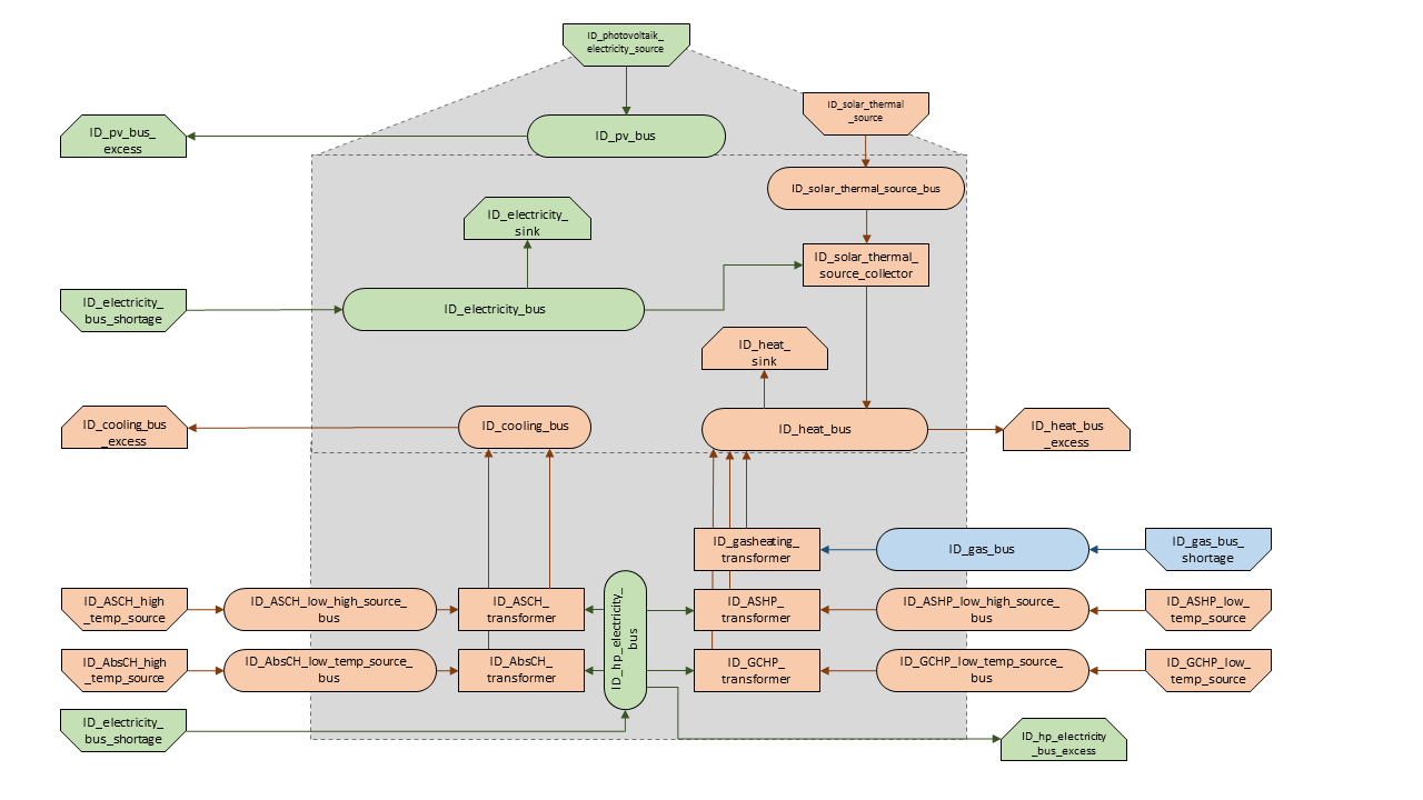
Graph of the energy system, which is created by entering the example components. The non-active components are not included in the graph above.
Storages
Within this sheet, the storages of the energy system are defined. The following parameters have to be entered:
label: Unique designation of the storage. Also for storages that are not activated. The following format is recommended: “<ID>_<energy sector>_storage”. <ID> and <energy sector> need to be replaced by the storage attributes.
comment: Space for an individual comment, e.g. an indication of which measure this component belongs to.
active: Specifies whether the storage shall be included to the model. “0” = inactive, “1” = active.
storage type: Defines whether the storage is a “Generic” or a “Stratified” storage. These two inputs are possible.
input: Specifies the input of the storage. If the storage has only one connection, the same bus can be provided for input and output.
output: Specifies the output of the storage. If the storage has only one connection, the same bus can be provided for input and output.
input/capacity ratio (invest): Indicates the performance with which the storage can be charged (see also here).
output/capacity ratio (invest): Indicates the performance with which the storage can be discharged (see also here).
efficiency inflow: Specifies the charging efficiency.
efficiency outflow: Specifies the discharging efficiency.
initial capacity: Specifies how far the storage is loaded at time 0 of the simulation. Value must be between “0” and “1”. The initial capacity value must be equal or higher than the ‘capacity min’ value.
capacity min: Specifies the minimum amount of storage that must be loaded at any given time. Value must be between “0” and “1”.
capacity max: Specifies the maximum amount of storage that can be loaded at any given time. Value must be between “0” and “1”.
sector: This column is used to differentiate between an electricity, heat and cooling storages for the result processing energy amount collection. Possible entries: “electricity”, “heat”, “cooling”, “central_electricity”, “central_heat”, “central_cooling”.
Costs
existing capacity in (kW): Existing capacity of the storage before possible investment.
min. investment capacity in (kW): Minimum storage capacity to be installed.
max. investment capacity in (kW): Maximum in addition to existing capacity, installable storage capacity.
variable input costs in (CU/kWh): Indicates how many costs arise for charging with one kWh.
variable output costs in (CU/kWh): Indicates how many costs arise for charging with one kWh.
variable input constraint costs in (CU/kWh): Indicates how many costs arise for charging with one kWh referring to the constraint limit set in the “energysystem” sheet. If not considering constraints fill character “0” is used.
variable output constraint costs in (CU/kWh): Indicates how many costs arise for charging with one kWh referring to the constraint limit set in the “energysystem” sheet. If not considering constraints fill character “0” is used.
periodical costs in (CU/a): Costs incurred per kW for investments within the time horizon. Periodical costs only apply for newly invested capacities but not for existing capacities.
periodical constraint costs in (CU/a): Costs incurred per kW for investments within the time horizon referring to the constraint limit set in the “energysystem” sheet. If not considering constraints fill character “0” is used.
non-convex investment: Specifies whether the investment capacity should be defined as a mixed-integer variable, i.e. whether the model can decide whether NOTHING OR THE INVESTMENT should be implemented. Explained here.
fix investment costs in (CU/a): Fixed costs of non-convex investments (in addition to the periodic costs).
fix investment constraint costs in (CU/a): Fixed constraint costs of non-convex investments (in addition to the periodic costs).
Generic Storage
capacity loss: Indicates the storage loss per time unit where “0,03” represents 3 % daily losses. Only required, if the “storage type” is set to “Generic”.
Stratified Storage
diameter in (m): Defines the diameter of a stratified thermal storage, which is necessary for the calculation of thermal losses.
temperature high in (°C): Outlet temperature of the stratified thermal storage.
temperature low in (°C): Inlet temperature of the stratified thermal storage.
U value in (W/(m2 K)): Thermal transmittance coefficient.
label |
comment |
active |
storage type |
bus |
input/capacity ratio |
output/capacity ratio |
efficiency inflow |
efficiency outflow |
initial capacity |
capacity min |
capacity max |
existing capacity |
min. investment capacity |
max. investment capacity |
non-convex investment |
fix investment costs |
variable input costs |
variable output costs |
periodical costs |
variable input constraint costs |
variable output constraint costs |
periodical constraint costs |
capacity loss |
diameter |
temperature high |
temperature low |
U value |
sector |
|---|---|---|---|---|---|---|---|---|---|---|---|---|---|---|---|---|---|---|---|---|---|---|---|---|---|---|---|---|
(invest) |
(invest) |
(kWh) |
(kWh) |
(kWh) |
(CU/a) |
(CU/kWh) |
(CU/kWh) |
(CU/(kWh a)) |
(CU/kWh) |
(CU/kWh) |
(CU/(kWh a)) |
Generic Storage |
(m) | Stratified Storage |
(°C) | Stratified Storage |
Stratified Storage |
(W/(m2 K)) | Stratified Storage |
||||||||||||
ID_battery_storage |
1 |
Generic |
ID_electricity_bus |
0.17 |
0.17 |
1 |
0.98 |
0.1 |
0.1 |
1 |
0 |
0 |
100 |
0 |
0 |
0 |
0 |
70 |
0 |
0 |
400 |
0 |
0 |
0 |
0 |
0 |
electricity |
|
ID_thermal_storage |
1 |
Generic |
ID_heat_bus |
0.17 |
0.17 |
1 |
0.98 |
0.1 |
0.1 |
0.9 |
0 |
0 |
100 |
0 |
0 |
0 |
20 |
35 |
0 |
0 |
100 |
0 |
0 |
0 |
0 |
0 |
heat |
|
ID_stratified_thermal_storage |
0 |
Stratified |
ID_heat_bus |
0.2 |
0.2 |
1 |
0.98 |
0.05 |
0.05 |
0.95 |
0 |
0 |
100 |
0 |
0 |
0 |
20 |
35 |
0 |
0 |
100 |
0 |
0.8 |
60 |
40 |
0.04 |
heat |
|
district_battery_storage |
0 |
Generic |
district_electricity_bus |
0.17 |
0.17 |
1 |
0.98 |
0.1 |
0.1 |
1 |
0 |
0 |
1000 |
0 |
0 |
0 |
0 |
10 |
0 |
0 |
10 |
0 |
0 |
0 |
0 |
0 |
central_electricity |
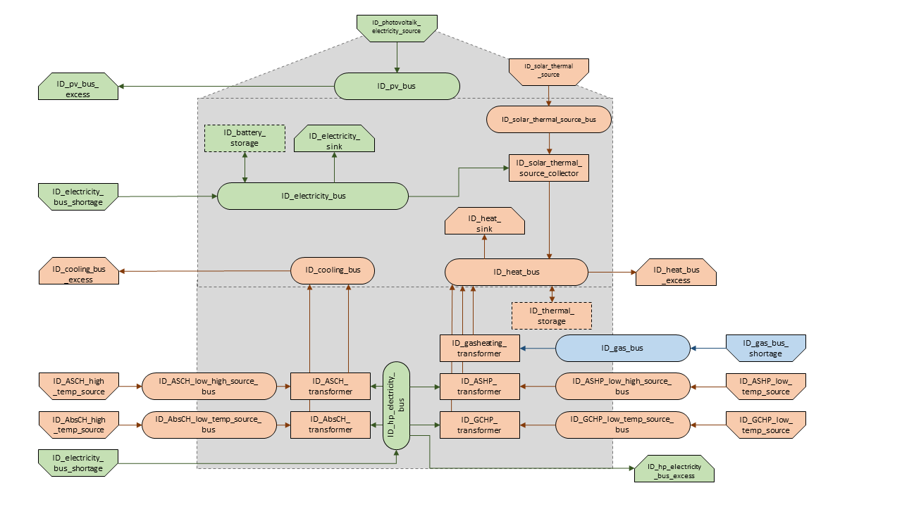
Graph of the energy system, which is created after entering the example components. The non-active components are not included in the graph above.
Links
Within this sheet, the links of the energy system are defined. The following parameters have to be entered:
label: Unique designation of the link. Also for links that are not activated. The following format is recommended: “<ID>_<energy sector>_link”. <ID> and <energy sector> need to be replaced by the link attributes.
comment: Space for an individual comment, e.g. an indication of which measure this component belongs to.
active: Specifies whether the link shall be included to the model. “0” = inactive, “1” = active.
bus1: First bus to which the link is connected. If it is a directed link, this is the input bus.
bus2: Second bus to which the link is connected. If it is a directed link, this is the output bus.
(un)directed: Specifies whether it is a directed or an undirected link. Input options: “directed”, “undirected”.
efficiency: Specifies the efficiency of the link. Values between 0 and 1 are allowed entries.
timeseries: Specifies whether the maximum transport capacity is limited by a timeseries in the Time series sheet or not. “0” = no timeseries, “1” = timeseries
Costs
existing capacity in (kW): Existing capacity of the link before possible investment.
min. investment capacity in (kW): Minimum, in addition to existing capacity, installable capacity.
max. investment capacity in (kW): Maximum capacity to be installed.
variable output costs in (CU/kWh): Indicates how many costs arise for transporting one kWh.
variable output constraint costs in (CU/kWh): Constraint costs incurred per kWh referring to the constraint limit set in the “energysystem” sheet. If not considering constraints fill character “0” is used.
periodical costs in (CU/(kW a)): Costs incurred per kW for investments within the time horizon. Periodical costs only apply for newly invested capacities but not for existing capacities.
periodical constraint costs in (CU/(kW a)): Costs incurred per kW for investments within the time horizon referring to the constraint limit set in the “energysystem” sheet. If not considering constraints fill character “0” is used.
non-convex investment: Specifies whether the investment capacity should be defined as a mixed-integer variable, i.e. whether the model can decide whether NOTHING OR THE INVESTMENT should be implemented. Explained here.
fix investment costs in (CU/a): Fixed costs of non-convex investments (in addition to the periodic costs).
fix investment constraint costs in (CU/a): Fixed constraint costs of non-convex investments (in addition to the periodic constraint costs).
label |
comment |
active |
timeseries |
(un)directed |
bus1 |
bus2 |
efficiency |
existing capacity |
min. investment capacity |
max. investment capacity |
non-convex investment |
fix investment costs |
variable output costs |
periodical costs |
variable constraint costs |
periodical constraint costs |
|---|---|---|---|---|---|---|---|---|---|---|---|---|---|---|---|---|
(kW) |
(kW) |
(kW) |
(CU/a) |
(CU/kWh) |
(CU/(kW a)) |
(CU/kWh) |
(CU/(kW a)) |
|||||||||
ID_pv_to_ID_electricity_link |
1 |
0 |
directed |
ID_pv_bus |
ID_electricity_bus |
1 |
0 |
0 |
0 |
0 |
0 |
0 |
0 |
0 |
0 |
|
ID_electricity_to_ID_hp_electricity_bus |
1 |
0 |
directed |
ID_electricity_bus |
ID_hp_electricity_bus |
1 |
0 |
0 |
0 |
0 |
0 |
0 |
0 |
0 |
0 |
|
district_heat_directed_link |
0 |
0 |
directed |
district_heat_bus |
ID_heat_bus |
0.85 |
0 |
0 |
0 |
0 |
0 |
0 |
0 |
0 |
0 |
|
district_heat_undirected_link |
0 |
0 |
undirected |
district_heat_bus |
ID_heat_bus |
0.85 |
0 |
0 |
0 |
0 |
0 |
0 |
0 |
0 |
0 |
|
district_electricity_link |
0 |
0 |
directed |
district_electricity_bus |
ID_electricity_bus |
1 |
0 |
0 |
0 |
0 |
0 |
0.1438 |
0 |
0 |
0 |
|
district_chp_to_district_electricity_bus |
0 |
0 |
directed |
district_chp_electricity_bus |
district_electricity_bus |
1 |
0 |
0 |
0 |
0 |
0 |
0.1438 |
0 |
0 |
0 |
|
ID_pv_to_district_electricity_link |
0 |
0 |
directed |
ID_pv_bus |
ID_electricity_bus |
1 |
0 |
0 |
0 |
0 |
0 |
0.1438 |
0 |
0 |
0 |
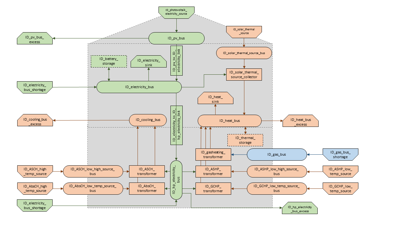
Graph of the energy system, which is created by entering the example components. The non-active components are not included in the graph above.
Insulation
Within this sheet, the energy system insulation options are defined. The following parameters have to be entered:
label: Unique designation of the insulation. Also for insulations that are not activated. The following format is recommended: “<ID>_<sink_label>_<insulation_type>”. <ID>, <sink_label> and <insulation_type> need to be replaced by the insulation attributes.
comment: Space for an individual comment, e.g. an indication of which measure this component belongs to.
active: Specifies whether the insulation shall be included to the model. “0” = inactive, “1” = active.
existing: Existing represents a boolean decision (“0” = no, “1” = yes). If a “1” is filled in here, the insulation measure is completely implemented without incurring any costs.
sink: Sink influenced by the insulation.
temperature indoor in (°C): Definition of the living space temperature.
heat limit temperature in (°C): Temperature from which the heating is switched on.
U-value old in (W/(m2 K)): U-value before insulation.
U-value new in (W/(m2 K)): U-value after insulation.
area in (m2): Area that can be considered for isolation.
periodical costs in (CU/(m2 *a)): Costs incurred per m2 for investments within the time horizon.
periodical constraint costs in (CU/(m2 *a)): Costs incurred per m2 for investments within the time horizon referring to the constraint limit set in the “energysystem” sheet. If not considering constraints fill character “0” is used.
label |
comment |
active |
existing |
sink |
temperature indoor |
heat limit temperature |
U-value old |
U-value new |
area |
periodical costs |
periodical constraint costs |
|---|---|---|---|---|---|---|---|---|---|---|---|
(°C) |
(°C) |
(W/(m2 K)) |
(W/(m2 K)) |
(m2) |
(CU/(m2)) |
(CU/(m2)) |
|||||
ID_heat_sink_window |
1 |
0 |
ID_heat_sink |
20 |
15 |
2.8 |
0.825 |
157.35 |
2400 |
21.9 |
Time Series
Within this sheet, time series and time-dependent price series, are stored. Time series are specified for components for which no automatically generated time series exist. These can be sinks to which the property “load profile” has been assigned as “time series” and sources with the “technology” property “time series”. Time-dependent price series are specified for buses with excess sinks or shortage sources where each period has a different price. These can be buses to which the property “excess costs” or “shortage costs” has been assigned as “timeseries”. The following parameters must be entered:
timestamp: Points in time to which the stored time series are related. The timestamps in the time series refer to local time, allowing the use of real measured data. On the days of the time change, specifically March 28 and October 28, there are special cases. On March 28, the clock is set forward from 2:00 AM to 3:00 AM, which means the hour between 2:00 and 2:59 AM does not exist in local time and is therefore missing in the data. On October 28, the clock is set back from 3:00 AM to 2:00 AM, causing the hour between 2:00 and 2:59 AM to occur twice (for the example of 2012). This results in a duplicated time span in the data for that hour. These effects arise from switching between daylight saving time and standard time. When working with local times, these missing or repeated hours must be taken into account to ensure data consistency. .
timeseries: Time series of a sink or a source which has been assigned the property “timeseries” under the attribute “load profile” or “technology. Time series contain a value between 0 and 1 for each point in time, which indicates the proportion of installed capacity accounted for by the capacity produced at that point in time. In the header line, the name must rather be entered in the format “componentID.fix” if the component enters the power system as a fixed component or it requires two columns in the format “componentID.min” and “componentID.max” if it is an unfixed component. The columns “componentID.min/.max” define the range that the solver can use for its optimization.
price series: Price Series of a bus with excess sink or shortage source which has been assigned the property “timeseries” under the attribute “excess costs” or “shortage costs”. In the header line, the name must be entered in the format “componentID.excess” for buses with excess sinks and “componentID.shortage” for buses with shortage sources. It is possible for a bus to have time-dependent price series in both a excess sink and a shortage source.
timestamp |
residential_electricity_demand.actual_value |
fixed_timeseries_electricty_source.fix |
unfixed_timeseries_electricty_source.min |
unfixed_timeseries_electricty_source.max |
fixed_timeseries_electricity_sink.fix |
unfixed_timeseries_electricity_sink.min |
unfixed_timeseries_electricity_sink.max |
fixed_timeseries_cooling_demand_sink.fix |
bus.excess |
bus.shortage |
|---|---|---|---|---|---|---|---|---|---|---|
2012-01-01 00:00:00 |
0.559061982 |
0.000000 |
0.000000 |
1.000000 |
0.000000 |
0.000000 |
1.000000 |
100 |
-0.1156 |
0.1156 |
2012-01-01 01:00:00 |
0.533606486 |
0.041667 |
0.000000 |
0.500000 |
0.041667 |
0.000000 |
0.500000 |
100 |
-0.1034 |
0.1034 |
2012-01-01 02:00:00 |
0.506058757 |
0.083333 |
0.000000 |
0.333333 |
0.083333 |
0.000000 |
0.333333 |
100 |
-0.09656 |
0.09656 |
2012-01-01 03:00:00 |
0.504140877 |
0.125000 |
0.000000 |
0.250000 |
0.125000 |
0.000000 |
0.250000 |
100 |
-0.09764 |
0.09764 |
2012-01-01 04:00:00 |
0.507104873 |
0.166667 |
0.000000 |
0.200000 |
0.166667 |
0.000000 |
0.200000 |
100 |
-0.09611 |
0.09611 |
2012-01-01 05:00:00 |
0.511376515 |
0.208333 |
0.000000 |
0.166667 |
0.208333 |
0.000000 |
0.166667 |
100 |
-0.10769 |
0.10769 |
2012-01-01 06:00:00 |
0.541801064 |
0.250000 |
0.000000 |
0.142857 |
0.250000 |
0.000000 |
0.142857 |
100 |
-0.12675 |
0.12675 |
2012-01-01 07:00:00 |
0.569261616 |
0.291667 |
0.000000 |
0.125000 |
0.291667 |
0.000000 |
0.125000 |
100 |
-0.13897 |
0.13897 |
2012-01-01 08:00:00 |
0.602998867 |
0.333333 |
0.000000 |
0.111111 |
0.333333 |
0.000000 |
0.111111 |
100 |
-0.13341 |
0.13341 |
2012-01-01 09:00:00 |
0.629064598 |
0.375000 |
0.000000 |
0.100000 |
0.375000 |
0.000000 |
0.100000 |
100 |
-0.12631 |
0.12631 |
Weather Data
If electrical load profiles are simulated with the Richardson tool, heating load profiles with the demandlib or photovoltaic systems with the feedinlib, weather data must be stored here. The weather data time system should be in conformity with the model’s time system, defined in the sheet “timesystem”.
timestamp: Points in time to which the stored weather data are related.
dhi in (W/m2): Diffuse horizontal irradiance.
dni in (W/m2): Direct normal irradiance.
ghi in (W/m2): Global horizontal irradiance.
pressure in (Pa): Air pressure.
temperature in (°C): Air temperature.
windspeed in (m/s): Wind speed, measured at 10 m height.
z0 in (m): Roughness length of the environment.
ground_temp in (°C): Constant ground temperature at 100 m depth.
water_temp in (°C): Varying water temperature of a river depending on the air temperature.
groundwater_temp in (°C): Constant temperature of the ground water at 6 - 10 m depth in North Rhine-Westphalia.
exergy_network_temp in (°C): Temperatur of the exergy network.
anergy_network_temp in (°C): Temperatur of the anergy network.
timestamp |
dhi |
dni |
ghi |
pressure |
temperature |
windspeed |
z0 |
ground_temp |
water_temp |
groundwater_temp |
exergy_network_temp |
anergy_network_temp |
|---|---|---|---|---|---|---|---|---|---|---|---|---|
2012-01-01 00:00:00 |
0.00 |
0.00 |
0.00 |
100672.78 |
10.03 |
5.33 |
0.49 |
13.7 |
14.62 |
13.06 |
90 |
15 |
2012-01-01 01:00:00 |
0.00 |
0.00 |
0.00 |
100678.25 |
10.36 |
5.13 |
0.49 |
13.7 |
14.62 |
13.06 |
90 |
15 |
2012-01-01 02:00:00 |
0.00 |
0.00 |
0.00 |
100680.18 |
10.57 |
4.99 |
0.49 |
13.7 |
14.71 |
13.06 |
90 |
15 |
2012-01-01 03:00:00 |
0.00 |
0.00 |
0.00 |
100651.83 |
10.67 |
4.93 |
0.49 |
13.7 |
14.75 |
13.06 |
90 |
15 |
2012-01-01 04:00:00 |
0.00 |
0.00 |
0.00 |
100618.33 |
10.81 |
4.86 |
0.49 |
13.7 |
14.99 |
13.06 |
90 |
15 |
2012-01-01 05:00:00 |
0.00 |
0.00 |
0.00 |
100594.81 |
10.73 |
5.26 |
0.49 |
13.7 |
14.97 |
13.06 |
90 |
15 |
2012-01-01 06:00:00 |
0.00 |
0.00 |
0.00 |
100558.41 |
10.83 |
5.39 |
0.49 |
13.7 |
14.96 |
13.06 |
90 |
15 |
2012-01-01 07:00:00 |
0.35 |
0.00 |
0.35 |
100566.46 |
11.10 |
5.79 |
0.49 |
13.7 |
15.17 |
13.06 |
90 |
15 |
2012-01-01 08:00:00 |
3.84 |
0.00 |
3.84 |
100572.26 |
11.14 |
5.86 |
0.49 |
13.7 |
15.46 |
13.06 |
90 |
15 |
2012-01-01 09:00:00 |
9.77 |
0.00 |
9.77 |
100568.07 |
11.26 |
5.99 |
0.49 |
13.7 |
15.57 |
13.06 |
90 |
15 |
2012-01-01 10:00:00 |
11.87 |
0.00 |
11.87 |
100560.02 |
11.63 |
5.79 |
0.49 |
13.7 |
15.44 |
13.06 |
90 |
15 |
… |
… |
… |
… |
… |
… |
… |
… |
… |
… |
… |
Pipe Types
Two different components are listed in this table. The first defines the different pipe types available to the energy system for the construction of heating networks and second the components which are the connection between the houses and the heat networks. These are the “dh_heatstation” for the exergy heat network and the “ anergy_heat_pump” for the anergy heat network.
label: Unique designation of the pipe types. Also for pipe types that are not activated. The following format is recommended for the pipes: “<DN>-<diameter of pipe>”.
active: Specifies whether the pipe type shall be included to the model. “0” = inactive, “1” = active.
nonconvex: Specifies whether the investment capacity should be defined as a mixed-integer variable, i.e. whether the model can decide whether NOTHING OR THE INVESTMENT should be implemented. Explained here.
loss factor: Proportional loss factor for the component.
loss factor fix: Fixed loss factor for the component.
min. investment capacity in (kW): Minimum capacity to be installed in case of an investment.
max. investment capacity in (kW): Maximum capacity that can be added in the case of an investment. If no investment is possible, enter the value “0” here.
periodical costs in (CU/(kW a)): Costs incurred per kW for investments within the time horizon. Periodical costs only apply for newly invested capacities but not for existing capacities.
fix investment costs in (CU/a): Fixed costs of non-convex investments (in addition to the periodic costs).
periodical constraint costs in (CU/(kW a)): Costs incurred per kW for investments within the time horizon referring to the constraint limit set in the “energysystem” sheet. If not considering constraints fill character “0” is used.
fix investment constraint costs in (CU/a): Fixed constraint costs of non-convex investments (in addition to the periodic constraint costs).
anergy or exergy: Specifies whether the pipe type is part of the anergy or exergy network. Fill in “exergy” for a pipe for an exergy network and “anergy” for a pipe of an anergy network.
distribution pipe: Specifies whether the pipe type can be used as a distribution pipe. Fill in “1” if the pipe type can be used and “0” if it cannot.
building pipe: Specifies whether the pipe type can be used as a building pipe. Fill in “1” if the pipe type can be used and “0” if it cannot.
efficiency: Specifies the efficiency of the first output. Values between “0” and “1” are allowed entries. This value is only relevant for the “dh_heatstation” and the “anergy_heat_pump”. A “0” can be inserted for the pipe types.
Exemplary input for pipe types label
active
nonconvex
loss factor
loss factor fix
min. investment capacity
max. investment capacity
periodical costs
fix investment costs
periodical constraint costs
fix investment constraint costs
anergy or exergy
distribution pipe
building pipe
efficiency
DN-20
0
1
0
0.010667
0
24.42
0
64
204
0
exergy
1
1
0
DN-25
0
1
0
0.012667
0
43.95
0
65
244
0
exergy
1
1
0
DN-32
0
1
0
0.015333
0
83.44
0
69
304
0
exergy
1
1
0
DN-40
0
1
0
0.017333
0
147.99
0
72
376
0
exergy
1
1
0
DN-50
0
1
0
0.019333
0
261.12
0
81
471.999847
0
exergy
1
1
0
DN-65
0
1
0
0.022
0
506.3
0
88
629
0.00001
exergy
0
1
0
DN-80
0
1
0
0.023333
0
851.92
0
101
800.999977
0.00001
exergy
1
0
0
DN-100
0
1
0
0.026
0
1490
0
125
1056
0
exergy
1
1
0
DN-125
0
1
0
0.028
0
2580
0
150
1412
0
exergy
1
1
0
DN-150
0
1
0
0.029333
0
4050
0
181
1812
0
exergy
1
1
0
DN-200
0
1
0
0.032
0
8220
0
215
2742
0
exergy
1
1
0
DN-250
0
1
0
0.034
0
14210
0
288
3844
0
exergy
1
1
0
Diameter65L
1
0
0.000022
0
0
9999
0.087724
0
0.627025
0
exergy
1
1
0
clustered_consumer_link
1
0
0
0
0
0
0.156558276
0
0.9122902
0
0
0
0
0.02898939
dh_heatstation
1
0
0
0
0
0
85
0
0.000001
0
0
0
0
0.98
anergy_heat_pump
1
0
0
0
0
0
1
0
1
0
0
0
0
1
Upscaling Tool
The Upscaling-Tool simplifies the creation of the model definition. For more information take a look at the method: Modeling Method.
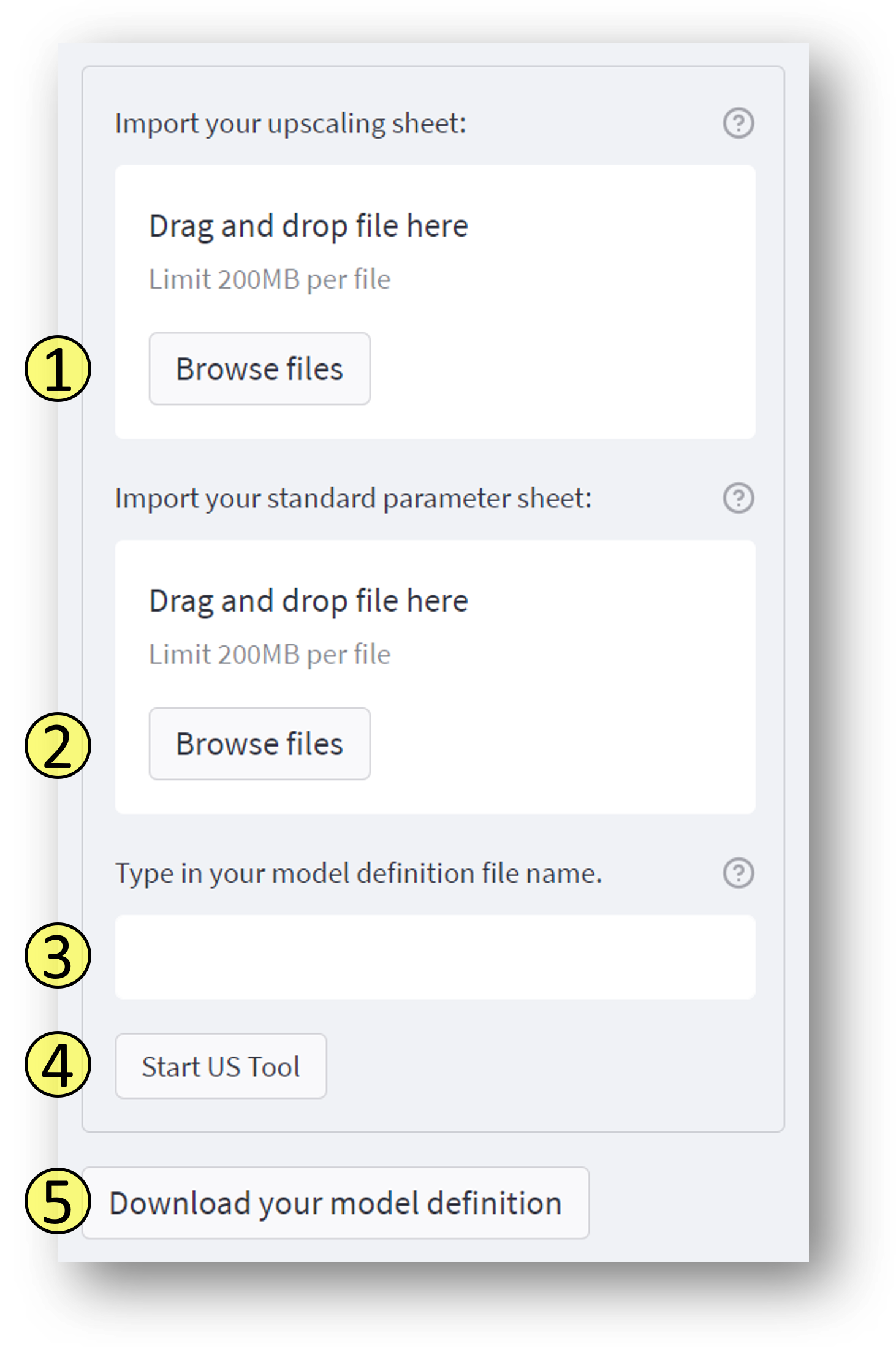
1. Uploading the upscaling sheet
Upload your upscaling_sheet.xlsx which contains all building-specific parameters.
2. Uploading the standard parameter sheet
Upload your standard_parameter.xlsx which contains all technological parameters.
3. Naming the model definition
You can choose any name for your model definition.
4. Starting the Upscaling-Tool
The model definition is created automatically and can be viewed on the right side.
5. Downloading the xlsx-file
If you agree with the model definition, it can be downloaded. The model definition serves as a basis for the optimization process and can be used on the Main Application.
Upscaling Sheet
This part of the documentation is taken from Budde’s master’s thesis [1] and guides how the upscaling sheet can be adapted.
Category 1
label |
comment |
active |
year of construction |
distance of electric vehicles |
electricity demand |
heat demand |
building type |
units |
occupants per unit |
gross building area |
latitude |
longitude |
year of construction wall |
area outer wall |
year of construction windows |
area windows |
year of construction roof |
rooftype |
area roof |
cluster ID |
flow temperature |
electricity cost |
heatpump electricity cost |
electricity emission |
heatpump electricity emission |
|---|---|---|---|---|---|---|---|---|---|---|---|---|---|---|---|---|---|---|---|---|---|---|---|---|---|
x |
km/a |
kWh / (sqm * a) |
kWh / (sqm * a) |
sqm |
° WGS 84 |
° WGS 84 |
sqm |
sqm |
sqm |
°C |
€/kWh |
g/kWh |
€/kWh |
g/kWh |
|||||||||||
001_building |
1 |
1800 |
0 |
400 |
400 |
COM_Food |
1 |
1 |
100 |
52.000000 |
7.000000 |
1800 |
50 |
0 |
0 |
1967 |
flat roof |
25 |
0 |
60 |
standard |
standard |
standard |
standard |
|
002_building |
1 |
1800 |
0 |
0 |
0 |
MFB |
1 |
1 |
50 |
52.000000 |
7.000000 |
1979 |
100 |
1999 |
20 |
1993 |
flat roof |
50 |
0 |
60 |
standard |
standard |
standard |
standard |
|
003_building |
1 |
1800 |
10000 |
30 |
20 |
SFB |
1 |
1 |
120 |
52.000000 |
7.000000 |
1994 |
250 |
2001 |
125 |
1992 |
step roof |
125 |
0 |
40 |
standard |
standard |
standard |
standard |
label: The building name can be chosen by the user and is the identification number (ID) of a building. The ID must be unique for each building, because all the following columns are assigned to it.
comment: Space for an individual comment, e.g. an indication of which measure this component belongs to.
active: In this cell, users decide whether a building should be considered in the modeling.
year of construction: The year of construction of a building is relevant for the calculation of the heat demand.
distance of electric vehicles (km/a): The annual kilometers driven are used to create the charging profile of an electric car. The electricity demand for the electric car is considered separately from the building electricity demand.
electricity demand (kWh / (m² a)): The specific electricity demand is multiplied by the useful building area to calculate the annual demand. If the annual electricity demand is not available as a function of the building floor area, 1 m² must be entered for the building floor area.
heat demand (kWh / (m² a)): The specific heat demand is multiplied by the useful building area to calculate the annual demand. If the annual heat demand is not available as a function of the building floor area, 1 m² must be entered for the building floor area.
building type: The building usage influences the calculation of the energy demand and the selection of the load profile for buildings. The different building types can be found in the standard parameter documentation (see standard parameter). The following input values are valid: SFB, MFB, COM_Food, COM_Retail, COM_Office, COM_School, COM_Stable, COM_Sports, COM_Workshop, COM_Restaurant and COM_Hotel.
units: The number of housing units is required for calculating the heat demand of residential buildings.
occupants per unit: The occupants per housing unit are required to calculate the electricity demand of the households. If the occupants per housing unit are multiplied by the housing units, the number of occupants per building can be calculated. The summed occupants of all buildings represent the total modeled neighborhood residents and provide a good basis for validation with real data.
gross building area (m²): The gross building area is required to calculate the annual electricity and heat demand of commercial buildings and the heat demand of residential buildings. For this purpose, the gross building area is multiplied by the specific electricity and heat demand and a building area factor (see standard parameter). The building area factor depends on the building use and reduces the gross building area by non-usable areas such as the base areas of walls.
latitude (° WGS 84): The latitude of the building are required to connect the building to a heating network. In addition, the coordinates are used to obtain weather data for PV systems from an external database. The World Geodetic System 1984 (WGS 84) is used as a reference system.
longitude (° WGS 84): The longitude of the building are required to connect the building to a heating network. In addition, the coordinates are used to obtain weather data for PV systems from an external database. The World Geodetic System 1984 (WGS 84) is used as a reference system.
year of construction wall: The year of construction of a walls is relevant for the calculation of the savings potential of insulation measures. For each building, the U-value (also heat transfer coefficient) is obtained from the standard parameter sheet (see standard parameter), depending on the year of construction of the building. In the Energy Saving Ordinance 2014, U-values are defined to achieve the desirable efficiency level 1. These U-values can be maximally achieved in the modeling. The difference between current and minimum U-value is the possible saving of heat demand. The calculation is explained in the standard parameter documentation (see standard parameter).
area outer wall (m²): The external wall area is relevant for the calculation of insulation measures.
year of construction windows: The year of construction of windows is relevant for the calculation of the savings potential of insulation measures. For each building, the U-value (also heat transfer coefficient) is obtained from the standard parameter sheet (see standard parameter), depending on the year of construction of the building. In the Energy Saving Ordinance 2014, U-values are defined to achieve the desirable efficiency level 1. These U-values can be maximally achieved in the modeling. The difference between current and minimum U-value is the possible saving of heat demand. The calculation is explained in the standard parameter documentation (see standard parameter).
area windows (m²): The window area is relevant for the calculation of insulation measures.
year of construction roof: The year of construction of a roof is relevant for the calculation of the savings potential of insulation measures. For each building, the U-value (also heat transfer coefficient) is obtained from the standard parameter sheet (see standard parameter), depending on the year of construction of the building. In the Energy Saving Ordinance 2014, U-values are defined to achieve the desirable efficiency level 1. These U-values can be maximally achieved in the modeling. The difference between current and minimum U-value is the possible saving of heat demand. The calculation is explained in the standard parameter documentation (see standard parameter).
rooftype: The roof type is differentiated between flat roofs and step roofs. The roof type is relevant for the calculation of insulation measures.
area roof (m²): The roof areas are relevant for the calculation of insulation measures.
cluster ID: The cluster ID is used to spatially assign a building to a specific area. The area can be, for example, a settlement or neighborhood. The cluster ID is crucial for spatial clustering.
flow temperature (°C): The flow temperature may differ depending on the heating system. The flow temperature should not fall below the heat source temperature of a heat pump. If the outdoor temperature is 35 °C and the flow temperature is 30 °C, the air heat pump is switched off and an alternative technology is used for heat supply.
electricity cost (€/kWh): If the user wants to use a electricity purchase price that differs from the standard parameter (e.g. due to a green electricity tariff), this can be entered here. If not the user has to enter “standard”.
electricity emission (g/kWh): If the user wants to use a electricity purchase emission that differs from the standard parameter (e.g. due to a green electricity tariff), this can be entered here. If not the user has to enter “standard”.
heatpump electricity cost (€/kWh): If the user wants to use a heatpump electricity purchase price that differs from the standard parameter (e.g. due to a different heatpump tariff), this can be entered here. If not the user has to enter “standard”.
heatpump electricity emission (g/kWh): If the user wants to use a heatpump electricity purchase emission that differs from the standard parameter (e.g. due to a different heatpump tariff), this can be entered here. If not the user has to enter “standard”.
Category 2
label |
HS |
ashp |
gchp |
parcel ID |
oil heating |
gas heating |
battery storage |
thermal storage |
central heat |
electric heating |
wood stove |
aahp |
st 1 |
pv 1 |
roof area 1 |
surface tilt 1 |
azimuth 1 |
st 2 |
pv 2 |
roof area 2 |
surface tilt 2 |
azimuth 2 |
|---|---|---|---|---|---|---|---|---|---|---|---|---|---|---|---|---|---|---|---|---|---|---|
x |
(m²) |
(°) |
(°) |
(m²) |
(°) |
(°) |
||||||||||||||||
001_building |
1 |
no |
no |
no |
no |
no |
no |
no |
yes |
no |
yes |
yes |
no |
no |
0 |
0 |
0 |
no |
no |
0 |
0 |
0 |
002_building |
1 |
no |
no |
no |
no |
yes |
no |
no |
no |
no |
yes |
yes |
yes |
yes |
150 |
75 |
100 |
0 |
0 |
0 |
0 |
0 |
003_building |
1 |
yes |
yes |
GCHP25 |
no |
no |
yes |
yes |
yes |
no |
yes |
yes |
yes |
yes |
200 |
50 |
180 |
0 |
0 |
0 |
0 |
0 |
label: The building name can be chosen by the user and is the identification number (ID) of a building. The ID must be unique for each building, because all the following columns are assigned to it.
ashp: Air source heat pumps (ASHP) can be considered in the optimization of a building if the air-regenerated noise of the fans does not exceed the limits of the Technical Instructions on Noise Abatement (TA Lärm). There are already some ASHP on the market that meet the requirements.
gchp: Ground-coupled heat pumps are limited by the area required for geothermal collectors or probes. If there is a potential area for the GCHP, the so-called parcel must be assigned to the buildings.
parcel ID: The parcel ID assigns a potential area for GCHP to the buildings. On an additional auxiliary data sheet, users enter the parcel ID and the potential area.
heat extraction (kW/m): The extraction capacity of the geothermal probes or collectors is crucial for the performance of the heat pumps. The extraction rate should be determined specifically for the location.
oil heating, gas heating, electric heating, battery storage, thermal storage, wood stove, aahp: The technologies are not subject to restrictions and can be considered as an investment alternative.
central heat: If a heating network is available, a network connection can be considered as an investment alternative.
wood stove share: If a value between 0 and 1 is used as “wood stove share”, this share is separated from the main household heat demand and connected primarily to the wood stove. To avoid insolubility, this bus is also connected to the main heating bus of the considered building. If this division of the sink is not desired, “standard” should be used.
solar thermal share: If a value between 0 and 1 is used as “solar thermal share”, this share is separated from the main household heat demand and connected primarily to the solar thermal collector. To avoid insolubility, this bus is also connected to the main heating bus of the considered building. If this division of the sink is not desired, “standard” should be used.
st 1: In this column it is decided whether the roof potential area applies to solar thermal (ST) systems. Possible entries: yes or no.
pv 1: In this column it is decided whether the roof potential area applies to photovoltaic (PV) systems. Possible entries: yes or no. As soon as both systems are relevant for one area, an area competition arises, which is automatically considered.
roof area 1 (m²): The roof potential area of a building can be divided into several partial roof areas with respect to the radiation intensity. In total, users can add 30 partial roof areas.
surface tilt 1 (°): The surface tilt is decisive for the dimensioning of the solar systems and depends on the construction of the roof.
azimuth 1 (°): The azimuth is also critical to solar system sizing and depends on the orientation of the building.
Category 3
label |
comment |
active |
technology |
latitude |
longitude |
area |
dh_connection |
azimuth |
surface tilt |
flow temperature |
length of the geoth. probe |
heat extraction |
|---|---|---|---|---|---|---|---|---|---|---|---|---|
° WGS 84 |
° WGS 84 |
sqm |
° |
° |
°C |
m |
(kW / (m*a)) |
|||||
electricity_exchange |
1 |
electricity_exchange |
||||||||||
battery_storage |
1 |
battery |
||||||||||
ng_chp |
0 |
naturalgas_chp |
heat_input |
|||||||||
bg_chp |
0 |
biogas_chp |
heat_input |
|||||||||
pe_chp |
0 |
pellet_chp |
heat_input |
|||||||||
wc_chp |
1 |
woodchips_chp |
heat_input |
|||||||||
swhp |
0 |
swhp_transformer |
heat_input |
|||||||||
ashp |
0 |
ashp_transformer |
heat_input |
|||||||||
gchp |
free area needed |
1 |
gchp_transformer |
2500 |
heat_input |
100 |
0.0328 |
|||||
ng_heating |
0 |
naturalgas_heating_plant |
heat_input |
|||||||||
bg_heating |
0 |
biogas_heating_plant |
heat_input |
|||||||||
pe_heating |
0 |
pellet_heating_plant |
heat_input |
|||||||||
wc_heating |
1 |
woodchips_heating_plant |
heat_input |
|||||||||
thermal_storage |
1 |
thermal_storage |
heat_input |
|||||||||
p2g |
0 |
power_to_gas |
heat_input |
|||||||||
heat_input |
heat center |
1 |
heat_input_bus |
52 |
7 |
40 |
||||||
central_pv_st |
free area needed |
1 |
pv&st |
52 |
7 |
15000 |
heat_input |
180 |
22.5 |
|||
screw_turbine |
1 |
timeseries_source |
label: The technology name can be chosen arbitrarily by the user and represents the ID of a central technology. The ID must be unique for each technology, because all following columns are assigned to it.
comment: Space for an individual comment, e.g. an indication of which measure this component belongs to.
active: In this cell, users decide whether a technology should be considered in the modeling.
technology: In this cell, the central technologies are considered (see table below).
latitude, longitude (° WGS 84): The WGS 84 coordinates are required when heat grid centers or ground-mounted solar systems are selected as technologies. The coordinates are used to locate the technologies.
area (m²): This is where the area for central solar and GCHP systems is entered.
dh_connection: In this cell, the central heat supply technologies are connected to a heat network center. The label of the heat network center must be entered. In addition, the corner points of the street pipes must be located in the auxiliary data sheet. Two WGS 84 coordinates are required for each corner point. The length of the house connection lines (distance between distribution line and house connection point) is calculated automatically. With the perpendicular point method, the shortest path for the house connection lines is always calculated. Twelve different pipe diameters are stored in the standard parameter sheer (see standard parameter), which can be considered as investment alternatives.
azimuth (°): For ground-mounted solar systems, the azimuth must be specified.
surface tilt (°): For ground-mounted solar systems, the surface tilt must be specified.
flow temperature (°C): For each heat network center, it is necessary to specify the flow temperature at which the technologies feed into the heat network.
length of the geoth. probe (m): For GCHP systems it is necessary to specify the length of the vertical heat exchanger.
heat extraction (kW / (m*a)): For GCHP systems it is necessary to specify the heat extraction for the heat exchanger.
key word |
meaning |
|---|---|
electricity_exchange |
local energy market |
battery |
battery storage |
naturalgas_chp |
natrual gas combined heat and power (CHP) |
biogas_chp |
biogas CHP |
pellet_chp |
pellet CHP |
woodchips_chp |
woodchip CHP |
swhp_transformer |
surface water heat pump (SWHP) |
ashp_transformer |
ASHP |
gchp_transformer |
GCHP |
naturalgas_heating_plant |
natural gas heating plant |
biogas_heating_plant |
biogas heating plant |
pellet_heating_plant |
pellet heating plant |
woodchips_heating_plant |
woodchips heating plant |
thermal_storage |
central thermal storage |
power_to_gas |
Power-to-Gas system (electrolyzer; hydrogen storage; fuel cell; methanization; natural gas storage) |
heat_input_bus |
heat network center |
pv&st |
central photovoltaic or solar thermal system |
timeseries_source |
time series e.g. hydropower plants |
Category 4
timestamp |
dhi |
pressure |
temperature |
windspeed |
z0 |
dni |
ghi |
ground_temp |
water_temp |
groundwater_temp |
screw_turbine.fix |
electric_vehicle.fix |
|---|---|---|---|---|---|---|---|---|---|---|---|---|
01.01.2012 00:00 |
0 |
100119.3125 |
8.656125 |
5.9235 |
0.159 |
0 |
0 |
12.6 |
14.62006667 |
13.06 |
0.420911041 |
0 |
01.01.2012 01:00 |
0 |
100113.836 |
8.9435 |
6.455 |
0.159 |
0 |
0 |
12.6 |
14.62006667 |
13.06 |
0.420911041 |
0 |
01.01.2012 02:00 |
0 |
100102.5625 |
9.210125 |
6.8535 |
0.159 |
0 |
0 |
12.6 |
14.71342667 |
13.06 |
0.420911041 |
0 |
01.01.2012 03:00 |
0 |
100075.5 |
9.6415 |
7.318 |
0.159 |
0 |
0 |
12.6 |
14.75492 |
13.06 |
0.420911041 |
0 |
01.01.2012 04:00 |
0 |
100026.8555 |
9.9285 |
7.916 |
0.159 |
0 |
0 |
12.6 |
14.99350667 |
13.06 |
0.420911041 |
0 |
… |
… |
… |
… |
… |
… |
… |
… |
… |
… |
… |
… |
… |
timestamp: The time stamp is entered with an hourly accuracy for one year (8 760 time steps). All further time series are assigned to this time stamp.
temperature (°C), dhi (W/m²), dni (W/m²), ghi (W/m²), pressure (Pa), windspeed (m/s), z0 (m): The time series can be obtained from the Open Energy Platform via the Open Fred interface integrated in the SESMG. For this purpose, the year and the centroid of the neighborhood are specified in the Graphical User Interface (GUI). The outdoor temperature (temperature) serves as a heat source for ASHP, influences the performance of the PV systems and has an impact on the heat transfer of the building components. Diffuse horizontal irradiance (dhi), direct normal irradiance (dni) and global horizontal irradiance (ghi) are required for solar systems. The air pressure (pressure), wind speed (windspeed), and surface roughness (z0) are required for wind turbines. In addition, the air pressure influences the design of the PV systems. Alternatively, the time series can be taken from other sources and added to the upscaling sheet.
ground_temp: The ground temperature serves as a heat source for GCHP.
water_temp: The water temperature serves as a heat source for SWHP.
groundwater_temp: The ground-water temperature serves as a heat source for ground-water heat pumps (GWHP).
screw_turbine.fix: This is a dimensionless time series that indicates the relative utilization of the hydropower screw. Multiplication by the maximum electrical power gives the power per time step.
electric_vehicle.fix: The time series represents the charging power of an electric car. Each time series value is automatically multiplied by the annual kilometers driven and transferred to the model_definition.xlsx.
Standard Parameter Sheet
The standard parameter sheet contains all technology-specific data (costs, emissions, efficiencies) as well as all other data (e.g. specific energy requirements) required for energy system modeling. The parameters used are included in the following standard parameter documentation: https://doi.org/10.5281/zenodo.6974401
The documents contain all values, formulas and related sources used. The standard parameter documentation is intended to ensure the reproducibility of the results. The documentation is continuously updated.
References
[1] Budde J., Leitfaden zur Modellierung von Energiesystemen (2022), master thesis.
[2] Klemm, C., Budde J., Vennemann P., Model Structure for urban energy system optimization models, unpublished at the time of publication of this documentation, 2021.
Results
Warning
If a time series preparation algorithm was applied for the (main-)model, not every time-step of the model was modeled. This must be considered when analysing energy amounts. Simplifying, it can be assumed that the modeled amount of energy multiplied by the variable cost factor (see methods section) corresponds to the actual amount of energy over the entire period. Changes in the cost structure, on the other hand, are taken into account automatically.
Interactive Results
You will be automatically directed to this page after the optimization process (1) or you may want to analyze existing results (2) again.
1. Result processing after optimization process
The results differ depending on whether you used only one optimization criterion (a) or whether you did a multi-criteria optimization (b).
1a. Single-criteria optimization
In a single-criteria optimization, the costs, emissions, and energy demands of the neighborhood are displayed. In addition, you can view the system graph and all building-specific load profiles via the interactive results.
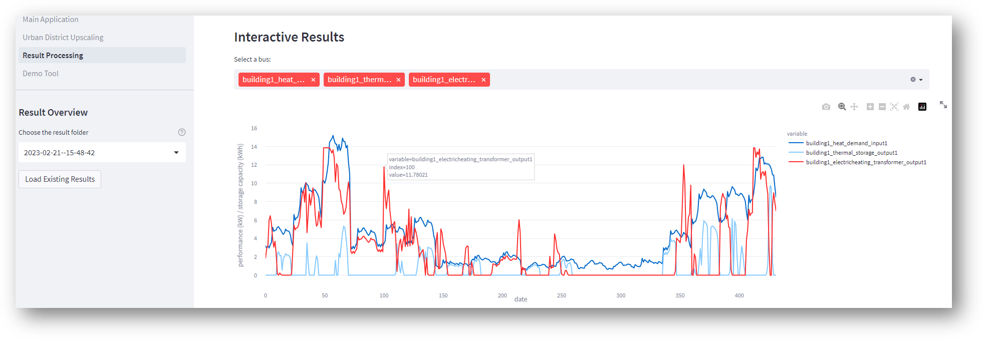
1b. Multi-criteria optimization
In multi-criteria optimization, several scenarios are calculated. For more information take a look at the method: Modeling Method. For each scenario, the results described for a single-criteria optimization can be displayed by selecting the reduction of the scenario (see (1) figure below). In addition, a Pareto diagram and energy amount diagrams are displayed (see (2) figure below).
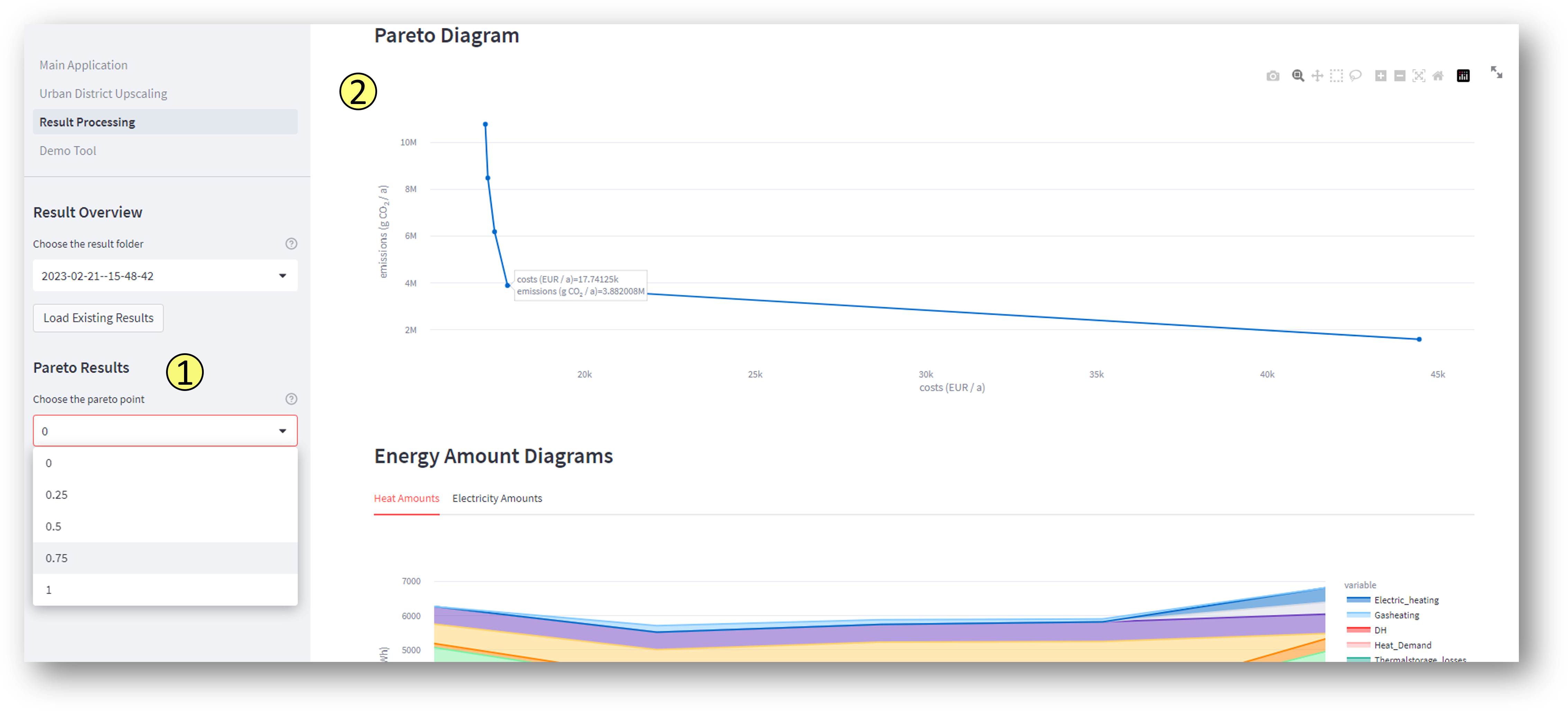
2. Result processing of existing results
The difference is that you need to select a folder that you want to analyze.
Results as Spreadsheets and Log-Files
The results of the modeling are stored in the SESMG result folder which is places by default in the /users/documents/SESMG/result directory. The directory is created by the SESMG application. You can change the directory when you are using the advanced installation by following the note information in the installation description.
- The results are saved in two formats:
as summarizing log files
as detailed xlsx-files and csv-files.
The log-file gives an overview of which components are created and which of the investment options should be implemented. The other files are explained in the following chapters. If you need more specified results, feel free to contact us as we have experience with different result summaries.
1. Results for a single-criteria optimization
1a. components.csv
The components.csv file provides detailed information about all components within the modeled energy system.
ID |
type |
input 1/kWh |
input 2/kWh |
output 1/kWh |
output 2/kWh |
capacity/kW |
variable costs/CU |
periodical costs/CU |
investment/kW |
max. invest./kW |
constraints/CU |
|---|---|---|---|---|---|---|---|---|---|---|---|
ID_electricity_bus_shortage |
source |
0 |
0 |
52.91 |
0 |
0.93 |
1158.78 |
0 |
0 |
0 |
1830873.62 |
This file includes key parameters such as energy flows, capacities, costs, investments, and constraints. Below is a description of each column in the file.
input 1/kWh and input 2/kWh: These columns represent the energy flows entering the component during the analyzed time period (if a timeseries simplification is selected this column contains only the summed up energy flows for the selected time frame).
output 1/kWh output 2/kWh: These columns capture the energy flows exiting the component during the specified time period (if a timeseries simplification is selected this column contains only the summed up energy flows for the selected time frame). If multiple outputs exist the order follows the description of the flows in the model definition.
- capacity/kW:
For non-storage components: This represents the maximum energy throughput, which is typically either the highest energy output or the highest energy input, measured in kilowatts (kW) for a one-hour period (see results.csv). This capacity can be either thermal or electrical, depending on the output 1 of the component. For most components this value is identical with the investment (exception for photovoltaic and solar thermal system).
For storage components: The capacity is represented in kilowatt-hours (kWh) instead of kilowatts (kW). This value indicates the total energy storage capacity of the component.
variable costs/CU and periodical costs/CU: These costs are expressed in Cost Units (CU) and are calculated for a one-year period. If a time series simplification is applied, these costs are scaled up for the whole year.
investment/kW: The investment corresponds to the actual usable power or the nominal power of the technology in kW.
max. invest./kW: This value is derived from the model definition and represents the upper investment limit of a specific component during the optimization process.
constraints/CU: Constraints are expressed in Cost Units (CU) and are typically calculated over a one-year period. If the constraint value is negative, and it refers to GHG (greenhouse gas) emissions, this indicates the reduction of emissions due to the usage of renewable energy sources, as per “consumption-based emission accounting”. If a time series simplification is applied, these costs are scaled up for the whole year.
1b. modified_model_definition.xlsx
The modified_model_definition is a copy of the sheets of the model definition that are potentially effected by a timeseries simplification. This includes the “weather data”, the “timeseries”, the “energysystem”, the “sinks” and the “buses”. The sheets “weather data” and “timeseries” contain all information about the weather or potential timeseries for each selected time step. If no timeseries simplification is selected, data for each hour of the year (8760 time steps) is displayed here.
1c. results.csv
For all components incoming and outgoing energy flows are specified for each time step of the model in kWh. The time steps include all hours of the year chosen by the timeseries simplification (if no timeseries simplification is chosen, results for each hour of the year are displayed).
1d. summary.cvs
The summary.csv contains the most important summarized results for the entire optimization.
Start Date |
End Date |
Resolution |
Total System Costs |
Total Constraint Costs |
Total Variable Costs |
Total Periodical Costs |
Total Energy Demand |
Total Energy Usage |
|---|---|---|---|---|---|---|---|---|
01.01.2012 |
05.01.2012 23:00 |
h |
4295.21 |
5481898.26 |
2736.69 |
1558.52 |
861.77 |
209.21 |
Total System Costs: The total costs over the course of a year, representing the sum of all variable costs (Total Variable Costs) and periodical costs (Total Periodical Costs).
Total Constraint Costs: The total constraint-related costs over the year (in the unit of the chosen constraint).
Total Variable Costs: Costs that vary depending on the energy quantities (these costs are not longer variable costs as they are already summed up for the whole year).
Total Periodical Costs: The sum of all periodical costs accumulated over the year.
Total Energy Demand: The demand represents the total amount of energy required by the various components of the energy system. In particular, the energy demanded by sinks (consumers) is recorded here (This value is not summed of for the entire year if a timeseries simplification is selected).
Total Energy Usage: The usage represents the amount of energy provided by the sources (Sources) in the system to meet the demand. Additionally, excess energy (Excess) is subtracted from Total Usage to reflect the actual energy consumption (This value is not summed of for the entire year if a timeseries simplification is selected).
1e. flow_information.cvs
The flow_information.csv file provides a detailed description of all flows listed in both the components.csv and the result table displayed in the GUI. It contains the name of each flow associated with each component, making it possible to distinguish between the different inputs and outputs (columns: Flow Input 1, Flow Input 2, Flow Output 1, Flow Output 2). For example, it becomes clear which input of a heat pump is associated with electricity.
2. Results for a Single-criteria optimization with district heating
If district heating is included in the optimization options additional result files are created.
The consumers_exergy and consumers_anergy files contain the consumers that are connected to the exergy or anergy network.
The producers_exergy and producers_anergy files contain the producers that are connected to the exergy or anergy network.
The files pipes_exergy and pipes_anergy contain the pipe sections of the energy and anergy network. The length of the pipes is included, as well the information which forks are connected.
The files forks_exergy and forks_anergy contain information abourt the coordinates of the forks of the networks. Forks are the junctions of the heat networks.
The file district_heating.jpeg provides a 2D view of the designed heating network. You can see the distribution network, the house connection pipes, the forks, consumers and producers.
3. Multi-criteria optimization
If a multi-criteria optimization is chosen each optimization run is saved with its specific results under the name of the model definition with the percentage of the constraint (0 for cost optimization, between 0 and 1 for the different Pareto points and 1 for the constraint cost optimization). The model_definitions with the constraint of the different runs (between 0 and one) are saved. Additionally, the following results are summarized for the different runs:
3a. elec_amounts.csv
This file contains the electricity amounts of the different optimization runs. The column “reductionco2” indicates the Pareto run, the “Electricity Demand” represents the total demand over the period of one year and the other columns represent the electricity outputs of the different components of the energy system. The unit of the electricity amounts is kWh.
3b. heat_amounts.csv
This file contains the heat amounts of the different optimization runs. The column “reductionco2” indicates the Pareto run, the “Heat Demand” represents the total demand over the period of one year and the other columns represent the heat outputs of the different components of the energy system. The unit of the heat amounts is kWh.
3c. pareto.csv
The file contains the summarized Total System Costs and Total Constraint Costs from the summary.csv of each run and is also used to display the Pareto front in the GUI.
Technical Data
Within the technical data section advanced model settings can be adjusted.
heuristic selection patterns
Within the ‘hierarchical_selection_schemes.xlsx’-file custom patterns for heuristic selection can be defined.
The xlsx-file contains an individual sheet for each applicable heursitic selection pattern. Each sheet is named with an integer number, which corresponds to the index with which the pattern can be selected during modeling. New patterns can be added as desired. Each pattern contains a list of reference periods, which are selected during the heuristic selection. The following information is stored for each reference period:
period: indicates from what period the reference period will be selected. Possible values are: year, winter, spring, summer, fall, integer number between 1 and 12.
criterion: indicates which parameter the selection of the reference period is based on. Possible values are: temperature, dhi, el_demand_sum, heat_demand_sum
value: indicates, whether the lowest, the highest or the most average value of the selected criterion within the selected period will be chosen. Possible values are: lowest, highest, average
average/extreme: indicates whether extreme values or average values of a reference period will be considered. For example, whether the period with the highest (value=highest) maximum (average/extreme=extreme) temperature (criterion=temperature) or the highest (value=highest) average (average/extreme=average) temperature (criterion=temperature) will be selected. Possible values are: extreme, average
characteristic_parameters
A database of absorption chillers has been created in the characteristic_parameters file. This can be extended by the user if required.
Warning
This database was taken from the examples of oemof thermal it is therefore not occupied by the developing team of the SESMG. A description of the parameters can be taken from oemof.thermal and papers by Ziegler.
Examples
For the SESMG, a number of examples can be found in this directory. Please make sure that the version indexed with the file/folder name matches your version of the SESMG. It is recommended to take a look at the mathematical graph theory before starting with the examples. Especially the terms sources, sinks, transformers, storages and buses should be understood. Further information can be found here. In the following, some examples are explained in more detail.
Example 1: Simulation and optimization of a single family house
The model definition template (“Task_1_template_model_definition.xlsx”) can be found in this directory of your version of the SESMG. There you will also find the completed model definition with solutions (“Task_1_solution_model_definition.xlsx”) as well as the graphical solutions. Your graphical results can be found directly in the Result Processing page at the menu point Energy System Graph. This example is intended as an introduction and has an exercise character.
The Müller family has three children and lives in a single-family house with 180 m2. They are planning to adapt the energy supply of their house. The entire heating demand of the family is currently provided by a gas heating system. To cover their electricity needs, the Müllers decided last year to install a PV system on the roof of the house. The rest of their electricity needs are met conventionally by connecting to the grid.
Known data:
Data |
Value |
|---|---|
Electricity Demand |
5 100 kWh |
Heat Demand |
32 000 kWh |
PV System |
5 kWp |
Simplification:
The PV system should be regarded as a new investment, as only a small portion of the depreciated to a small extent
Using the time series simplification “Slicing A” with 4 days (for hole example 1)
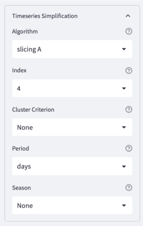
Simulation task:
Activate the given components via the column “active” as binary input. 0 = off, 1 = on
- Simulate the given energy system
To find out how to start a simulation, click here
Attention
After each change you have to save and upload the model definition again
Simulation: Min. and max. investment capacity identical. You use the same button for simulation as for optimization.
Example 1b: Cost optimization of the energy system
From the results of the simulation of the single-family house, it can be concluded that it makes sense to incorporate additional technologies in order to reduce the cost of energy supply. In this example, the following technologies are available:
Air source heat pump (ASHP) with max. 20 kW
Ground source heat pump (GCHP) with max. 15 kW
Battery storage with max. 10 kWh
Thermal storage with max. 20 kWh
Optimization task:
- Adjusts the templates of the individual technologies in the model definition accordingly and supplements them in the system
To find out how to start a optimization, click here
Attention
The electricity for a heat pump is purchased at a different price than the normal energy purchase. Therefore, two different buses are used.
Simulation (Example 1a): Min. and max. investment capacity identical
Optimization (Example 1b): Interval between min. and max. investment capacity
Example 1c: Pareto optimization of a single family house
The Müller family has heard that the emissions caused by energy systems can be significantly reduced by low additional costs.
Pareto-optimization task:
Execute a Pareto optimization of the energy system
Calculate the cost and emission minimums, as well three other Pareto points
Select the points in such a way that they are as meaningful as possible.
Attention
0 or 0 % represents the cost minimum, since 0 % of the possible emission reduction is exhausted
100 or 100 % represents the emission minimum, since 100 % of the possible emission reduction is utilized
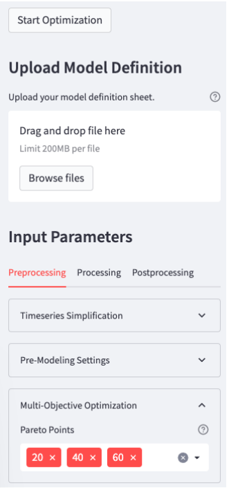
Pareto diagram:
This diagram is an example. Your Pareto curve should look similar.
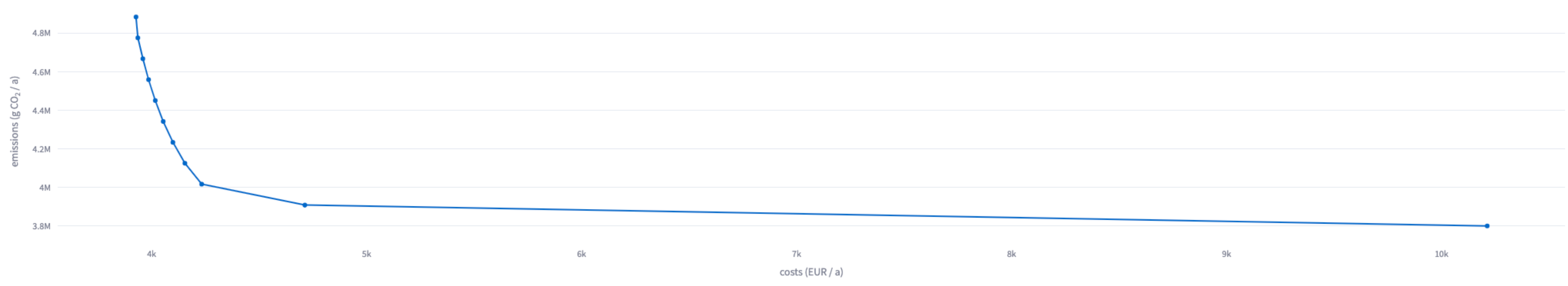
Example 2: Simulation and optimization of an industrial company
The model definition template (“Task_2_template_model_definition.xlsx”) can be found in this directory of your version of the SESMG. There you will also find the completed model definition with solutions (“Task_2_solution_model_definition.xlsx”) as well as the graphical solutions. Your graphical results can be found directly in the Result Processing page at the menu point Energy System Graph. This example is intended as an introduction and has an exercise character.
Schmiede GmbH manufactures various metal goods. It operates a property with several production halls. The systems have a high electricity demand. This follows the standard load profile “Gewerbe durchlaufend”(Commercial continuous) of the German Association of Energy and Water Industries (BDEW). The heat demand is negligible.
Known data:
Data |
Value |
|---|---|
Electricity Demand |
760 500 kWh |
Price of Electricity Purchase |
0.15 €/kWh |
Simplification:
Using the time series simplification “Slicing A” with 4 days (for hole example 2)
Simulation task:
Copy the sample components for operation and reconfigure them accordingly
- Simulate the given energy system
To find out how to start a simulation, click here
Note
The standard load profile is already stored in the SESMG. You can enter this under “sinks” - “load profile” as “g3”
further parameters (e.g. specific costs or emissions) are to be used from the example components for the same technologies
Example 2b: Optimization of an industrial company part I
Schmiede GmbH has sufficient land available for regenerative power generation on its own premises.
Two hall roofs are available to install PV systems:
Hall 1 with Sloped Roof
Parameter |
Value |
|---|---|
Orientation |
South-West |
Azimuth |
225° |
Surface tilt |
35° |
Roof Surface Reflectance (albedo) |
0.20 |
Max. Rated Power Output |
200 kW |
Hall 2 with Sloped Roof
Parameter |
Value |
|---|---|
Orientation |
East |
Azimuth |
100° |
Surface tilt |
27° |
Roof Surface Reflectance (albedo) |
0.18 |
Max. Rated Power Output |
150 kW |
Optimization task:
- Optimise the industrial company with new parameters
To find out how to start a optimization, click here
Note
Both units can be balanced and billed together
Create a separate sink for each PV system
One bus is sufficient for both PV systems
A separate link is necessary to connect the PV system to the local electricity bus
The surplus electricity can be sold at a tariff of 0.0635 €/kWh
Example 2c: Optimization of an industrial company part II
Next to the hall 1 of Schmiede GmbH there is a large open area. A wind turbine can be set up. A turbine from the manufacturer Vestas with a rotor diameter of 112 m and a hub height of 140 m was identified as principle suitable.
Optimization task:
Optimise the industrial company with new parameters
Search for a suitable model in the database and enter it in the same way in the table. The required data can be found in the subpackage “windpowerlib”.
Note
The surplus electricity can be sold at a tariff of 0.057 €/kWh
The wind turbine is designed (in this example) as a binary decision. This means that it is is either designed completely or not at all
To do this, you must create the plant as a “non-convex investment”. You activate this with 0 or 1 in the corresponding cell
The costs are summarised in a periodic cost of 100 €/kW*a
Example 2d: Optimization of an industrial company part III
The entire vehicle fleet of Schmiede GmbH is to be electrified within the next 5 years. This will not change the driving behavior. The resulting load profile was determined in a preliminary study. This is available in standardized form. Schmiede GmbH has 16 vehicles. The charging power is assumed to be 10 kW.
Optimization task:
Optimise the industrial company with new parameters
Create the vehicle fleet as another consumer (sink)
Note
You can find the normalised time series here. Insert it into the worksheet “timeseries”. The column must have the same name as your sink with the addition .fix
Since this is a normalized time series, the “nominal value” of the sink must be determined on the basis of the maximum possible charging capacity of the vehicle fleet. To achieve this, create a single sink with a nominal value of 160 kW
Example 3: Simple example of a heating network
This example shows the implementation of a exergy heating network. Three houses are considered and connected to the heating network. Electricity supply technologies were neglected in this case to reduce complexity. A decentralised geothermal heat pump was added for each house as an investment alternative to the heating network. The heating network consists of two pipe sections. This example only illustrates the basic structure for implementing a heating network, but can be expanded as required with additional pipe sections, technologies and the number of houses to be connected. You will find the “model_definition_example_heat_network.xlsx” in the this directory of your version of the SESMG.
The following table shows how the buses must be set up to implement a heating network. In “district heating conn. (exergy)”, a “1” is entered to connect the bus to the heating network. The longitude and latitude of the house connection station are entered in the “lat” and “lon” columns. At the same time a bus (here: “district_heat_bus”) is created, representing the district heat station of the heating network. In “district heating conn. (exergy)” a “dh-system” is entered and in the columns “lat” and “lon” the coordinates of the district heating station are entered. The district heat station is the point at which the central heat supply technologies feed into the heating network. The house connection points and the district heating station are automatically connected to the distribution pipe by the shortest route.
label |
comment |
active |
excess |
shortage |
excess costs |
shortage costs |
excess constraint costs |
shortage constraint costs |
district heating conn. (exergy) |
lat |
lon |
existing heathouse station |
district heating conn. (anergy) |
flow temperature |
electricity bus |
sector |
|---|---|---|---|---|---|---|---|---|---|---|---|---|---|---|---|---|
(CU/kWh) |
(CU/kWh) |
(CU/kWh) |
(CU/kWh) |
(°) |
(°) |
(°C) |
||||||||||
ID_heat_bus_1 |
1 |
0 |
0 |
0 |
0 |
0 |
0 |
1 |
50.05 |
7.05 |
0 |
0 |
60 |
ID_hp_electricity_bus_1 |
heat |
|
ID_heat_bus_2 |
1 |
0 |
0 |
0 |
0 |
0 |
0 |
1 |
49.6 |
7 |
0 |
0 |
60 |
ID_hp_electricity_bus_2 |
heat |
|
ID_heat_bus_3 |
1 |
0 |
0 |
0 |
0 |
0 |
0 |
1 |
49.8 |
7.1 |
0 |
0 |
60 |
ID_hp_electricity_bus_3 |
heat |
|
district_heat_bus |
1 |
0 |
0 |
0 |
0 |
0 |
0 |
dh-system |
50 |
7 |
0 |
0 |
0 |
0 |
central_heat |
The following table shows how a road network is mapped as the basis for the distribution system of a heating network. For this purpose, the road sections are mapped via the starting point and the end point of the road. The coordinates are entered in the columns “lat. 1st intersection”, “lat. 2nd intersection”, “lon. 1st intersection”, “lon. 2nd intersection”. The end point of the 1st intersection forms the start point of the 2nd intersection.
label |
comment |
lat. 1st intersection |
lat. 2nd intersection |
lon. 1st intersection |
lon. 2nd intersection |
active |
|---|---|---|---|---|---|---|
x |
x |
x |
x |
|||
ID_street1 |
49.30000 |
50.30000 |
6.80000 |
7.30000 |
1 |
|
ID_street2 |
50.30000 |
50.00000 |
7.30000 |
7.40000 |
1 |
The following table shows how the pipes used in the model are mapped for the heating network. In the “active” column, pipes with “1” are included in the model and pipes with “0” are not included in the model.
label |
active |
nonconvex |
loss factor |
loss factor fix |
min. investment capacity |
max. investment capacity |
periodical costs |
fix investment costs |
periodical constraint costs |
fix investment constraint costs |
anergy or exergy |
distribution pipe |
building pipe |
efficiency |
|---|---|---|---|---|---|---|---|---|---|---|---|---|---|---|
DN-200 |
0 |
1 |
0 |
0.032 |
0 |
8220 |
0 |
114 |
4112 |
0 |
exergy |
1 |
1 |
0 |
DN-250 |
1 |
1 |
0 |
0.034 |
0 |
14210 |
0 |
152 |
0 |
5765 |
exergy |
1 |
1 |
0 |
The heating network is displayed as a .jpeg in the results. The heating network shown in the example is illustrated in the following figure.

Anergy heating networks and Exergy heating networks differ in the temperature level. In Anergy heating networks, the temperature level is so low that a water-to-water heat pump is installed in the connected buildings to raise the temperature level. The cost of the heat pump is included in the cost of the house connection station of the Anergy heating network. Due to the low temperature level, uninsulated rather than insulated pipes are used in contrast to the Exergy heating network. There are only a few adjustments that need to be made in order to consider an Anergy heating network. The pipes for an Anergy heating network have to be defined in the “pipe types” sheet. In addition, the sheet “buses” is adapted in the same way as for the Exergy heating network. For this purpose, in the “district heating conn. (anergy)” column, enter a “1” if the bus is to be connected to the Anergy heating network and “dh-system” if the district heating station is to be defined.
label |
comment |
active |
excess |
shortage |
excess costs |
shortage costs |
excess constraint costs |
shortage constraint costs |
district heating conn. (exergy) |
lat |
lon |
existing heathouse station |
district heating conn. (anergy) |
flow temperature |
electricity bus |
sector |
|---|---|---|---|---|---|---|---|---|---|---|---|---|---|---|---|---|
(CU/kWh) |
(CU/kWh) |
(CU/kWh) |
(CU/kWh) |
(°) |
(°) |
(°C) |
||||||||||
ID_heat_bus_1 |
1 |
0 |
0 |
0 |
0 |
0 |
0 |
0 |
50.05 |
7.05 |
0 |
1 |
60 |
ID_hp_electricity_bus_1 |
heat |
|
ID_heat_bus_2 |
1 |
0 |
0 |
0 |
0 |
0 |
0 |
0 |
49.6 |
7 |
0 |
1 |
60 |
ID_hp_electricity_bus_2 |
heat |
|
ID_heat_bus_3 |
1 |
0 |
0 |
0 |
0 |
0 |
0 |
0 |
49.8 |
7.1 |
0 |
1 |
60 |
ID_hp_electricity_bus_3 |
heat |
|
district_heat_bus |
1 |
0 |
0 |
0 |
0 |
0 |
0 |
0 |
50 |
7 |
0 |
dh-system |
0 |
0 |
central_heat |
Example 4: Regular example of the documentation
This example is the basis for the documentation and explanation of the model definition. You can find the “v1.x_model_definition_example.xlsx” in the directory of your version of the SESMG.