Structure of Energy Systems
Energy systems in the sense of the Spreadsheet Energy System Model Generator are designed according to the specifications of the oemof library. Accordingly, energy systems can be represented with the help of mathematical graph theory. Thus, energy systems are exemplified as “graphs” consisting of sets of “vertices” and “edges”. In more specific terms, vertices stand for components and buses while directed edges connect them. The status variable of the energy flow indicates which amount of energy is transported between the individual nodes at what time. Possible components of an oemof energy system are
sources,
sinks,
transformers, and
storages.
Buses furthermore form connection points of an energy system. The graph of a simple energy system consisting of each one source, one transformer, one sink, as well as two buses, could look like the example displayed in the following figure.

Graph of a simple energy system, consisting of one source, two buses, one transformer, and one a sink.
An oemof energy system must be in equilibrium at all times. Therefore sources must always provide exactly as much energy as the sinks and transformer losses consume. In turn, the sink must be able to consume the entire amount of energy supplied. If there is no balance, oemof is not able to solve the energy system.
Buses
The modelling framework oemof does not allow direct connections between components. Instead, they must always be connected with a bus. The bus in turn can be connected to other components, so that energy can be transported via the bus. Buses can have any number of incoming and outgoing flows. Buses can not directly be connected with each other. They do not consider any conversion processes or losses.
Sources
Sources represent the provision of energy. This can either be the exploitation of an energy source (e.g. gas storage reservoir or solar energy, no energy source in physical sense), or the simplified energy import from adjacent energy systems. While some sources may have variable performances, depending on the temporary needs of the energy system, others have fixed performances, which depend on external circumstances. In the latter case, the exact performances must be entered to the model in form of time series. With the help of oemofs “feedinlib” and “windpowerlib”, electrical outputs of photovoltaic (PV)-systems and wind power plants can be generated automatically. In order to ensure a balance in the energy system at all times, it may be useful to add a “shortage” source to the energy system, which supplies energy in the event of an energy deficit. In reality, such a source could represent the purchase of energy at a fixed price.
Photovoltaic Systems
The following figure sketches the fractions of radiation arriving at a PV-module as well as further relevant parameters.

Radiation on a photovoltaic module.
The global radiation is composed of direct and diffuse radiation. The “direct horizontal irradiance” dirhi is the amount of sun radiation as directly received by a horizontal surface. The “diffuse horizontal irradiance” dhi is the share of radiation, which arrives via scattering effects on the same surface. A part of the global radiation is reflected on the ground surface and can thus cause an additional radiation contribution on the photovoltaic module. The amount of the reflected part depends on the magnitude of the albedo of the ground material. Exemplary albedo values are listed in the following table.
Material |
Consumer Group |
|---|---|
herbage (july, august) |
0.25 |
pasture |
0.18 - 0.23 |
uncoppied fields |
0.26 |
woods |
0.05 - 0.18 |
heath area |
0.10 - 0.25 |
asphalt |
0.15 |
concrete, clean |
0.30 |
concrete, weathered |
0.2 |
snow cover, fresh |
0.80 - 0.90 |
snow cover, old |
0.45 - 0.70 |
Wind Turbines
For the modeling of wind turbines, the weather data set must include wind speeds, as well as the roughness length z0 and the pressure. The wind speeds must be available for a measurement height of 10 m in the unit m/s.
The system data of the wind turbine to be modelled are obtained from the “oedb” database.
Solar thermal collectors
There are two collector types that can be modeled with this function.
flat plate collectors
concentrated solar power (parabolic through collector)
The irradiance on the flat plate collector is very similar to the photovoltaic source, although the reflected irradiance and the albedo are not a part of the calculation for flat plate collectors. For visualization you can take a look at the graph above.
The heat output of a parabolic through collector is based on the direct horizontal irradiance, the diffuse irradiance is not absorbed.
The solar thermal collector function automatically creates a heat source, a collector bus object and a transformer object. The output of the source is the actual heat, the collector would produce due to its technical parameters. The transformer object embodies the systems periphery (pipes, pumps). Thermal losses and the electricity demand of this periphery can be considered by the transformer.
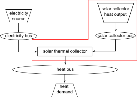
Graph of a solar thermal collector system.
The irradiance on the collector, its efficiency and the heat output is calculated by using “oemof.thermal”. Therefore specific values have to be given. Eta 0 is the optical efficiency of the collector, A1 is the linear heat loss coefficient and A2 is the quadratic heat loss coefficient. Values for Eta 0, A1 and A2 are collector specific values and can be found in data sheets. These values are measured and calculated according to DIN EN ISO 9806. The parameters C1 and C2 for concentrated solar power are collector specific values as well. An exemplary set of values is given in the documentation on how to use the model definition file.
The solar irradiance is given in W/sqm. Therefore the collector’s heat output is given in this unit as well. The investment object has to be power (kW). So the energy output (kW/sqm) has to be multiplied with a conversion factor. The conversion factor (sqm/kW) is calculated by dividing the gross aperture area of a collector model by a measured power output per module, e.g at 1000 W/sqm (DIN EN ISO 9806).
Some data sheets doesn’t contain all the necessary data. So another useful tool is the “Keymark Certificate Database”. The Keymark Certificate of a flat plate collector contains measured collector specific test data (a1, a2, eta 0, different power outputs).
Example: “Keymark Certificate 011-7S2432 F”. If this collector is part of the energy model, the conversion factor is calculated by dividing the gross aperture area (2,53 sqm) by the power output. Considering an average inside collector temperature of 40 °C and an outside average temperature of 10 °C result in a temperature difference of 30 K. So, in this case the heat power output is 1,504 kW and the conversion factor roundabout 1,68 (sqm/kW).
Power output per collector module |
||||||||||
|---|---|---|---|---|---|---|---|---|---|---|
G=1000W/sqm |
||||||||||
Aperture area (Aa) |
Gross length |
Gross width |
Gross heigth |
Gross area (AG) |
Tm-Ta |
|||||
0K |
10K |
30K |
50K |
70K |
||||||
Collector name |
sqm |
mm |
mm |
mm |
sqm |
W |
W |
W |
W |
W |
Flachkollektor FK 253 HA-4A |
2.34 |
2104 |
1204 |
80 |
2.53 |
1808 |
1712 |
1504 |
1278 |
1032 |
Example for calculation of conversion factor.
Note
If you are calculating a system with the concentrated solar power module, you need to be careful. Depending on the azimuth of the system some tests have shown, that for some hours of the considered period the calculated power output of the concentrated solar power module peaks by a factor of e.g. 100 compared to the rest of the period. This was observed with increasing azimuth e.g. an azimuth of 270 degrees. These peaks in power output are not possible, so the final results have to be evaluated carefully. The interactive results in the end can help to identify possible peaks very well.
Sinks
Sinks represent either energy demands within the energy system or energy exports to adjacent systems. Like sources, sinks can either have variable or fixed energy demands. Sinks with variable demands adjust their consumption to the amount of energy available. This could for example stand for the sale of surplus electricity. However, actual consumers usually have fixed energy demands, which do not respond to amount of energy available in the system. As with sources, the exact demands of sinks can be passed to the model with the help of time series.
In order to ensure a balance in the energy system at all times, it may be appropriate to add an “excess” sink to the energy system, which consumes energy in the event of energy surplus. In reality, this could be the sale of electricity or the give-away of heat to the atmosphere.
Standard Load Profiles
Oemof’s sub-library demandlib can be used for the estimation of heat and electricity demands of different consumer groups, as based on German standard load profiles (SLP). The following electrical standard load profiles of the Association of the Electricity Industry (VDEW) can be used:
Profil |
Consumer Group |
|---|---|
h0 |
households |
g0 |
commercial general |
g1 |
commercial on weeks 8-18 h |
g2 |
commercial with strong consumption in the evening |
g3 |
commercial continuous |
g4 |
shop/hairdresser |
g5 |
bakery |
g6 |
weekend operation |
l0 |
agriculture general |
l1 |
agriculture with dairy industry/animal breeding |
l2 |
other agriculture |
The following heat standard load profiles of the Association of Energy and Water Management (BDEW) can be used:
Profile |
House Type |
|---|---|
efh |
single family house |
mfh |
multi family house |
gmk |
metal and automotive |
gha |
retail and wholesale |
gko |
Local authorities, credit institutions and insurance companies |
gbd |
other operational services |
gga |
restaurants |
gbh |
accommodation |
gwa |
laundries, dry cleaning |
ggb |
horticulture |
gba |
bakery |
gpd |
paper and printing |
gmf |
household-like business enterprises |
ghd |
Total load profile Business/Commerce/Services |
In addition, the location of the building and whether the building is located in a “windy” or “non-windy” area are taken into account for the application of heat standard load profiles. The following location classes may be considered:
Stochastic Load Profiles (Richardson Tool)
The use of standard load profiles has the disadvantage that they only represent the average of a larger number of households (> 200). Load peaks of individual households (e.g. through the use of hair dryers or electric kettles) are filtered out by this procedure. To counteract this, the Spreadsheet Energy System Model Generator offers the possibility to generate stochastic load profiles for residential buildings. These are generated on the basis of Richardsonpy. Thereby, an arbitrary number of different realistic load profiles is simulated under consideration of statistic rules. The mean value of a large-enough number of profiles should, again, result in the standard load profile. However, if calculations are continued using the individual values before averaging – as in the above calculation of costs – different values are obtained than when calculating with SLPs. Different stochastic load profiles are created with the same input values. The calculation is based on the annual energy demand and the number of occupants.
Transformers
Transformers are components with one ore more input flows, which are transformed to one or more output flows. Transformers may be power plants, energy transforming processes (e.g. electrolysis, heat pumps), as well as transport lines with losses. The transformers’ efficiencies can be defined for every time step (e.g. the efficiency of a thermal powerplants in dependence of the ambient temperature).
These may have one or more different outputs, e.g. heat and electricity. For the modelling, the nominal performance of a generic transformer with several outputs, the respective output ratios, and an efficiency for each output need to be known.
Compression Heat Transformers
For the modeling of compression heat pumps and chillers, different heat sources are considered so the weather data set must include different temperatures. The efficiency of the heat pump or chiller cycle process can be described by the coefficient of performance (COP). The compression heat transformer function automatically creates a heat source and a low or high temperature bus, depending on the mode of operation (see red bubble). So only a transformer and a electricity bus needs to be created. An example is shown in the following figure.
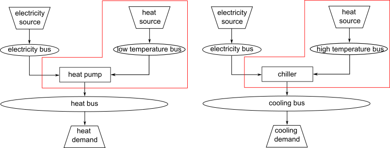
Graph of a compression heat pump (left) and compression chiller (right).
At the moment it is possible to use ground water, soil (vertical heat exchanger), surface water and ambient air as a heat source.
The compression heat transformers are implemented by using “oemof.thermal” .
Absorption Heat Transformers
At this point this function implies the modeling of an absorption chiller. An absorption chiller object contains a high temperature heat source, the necessary connection bus and a transformer object, that describes the absorption chiller. The heat source can be waste heat for example. The efficiency of the absorption chiller is described by the coefficient of Performance (COP).
The necessary parameters for the characteristic equation method are found in the “characteristic_parameters.csv” in the folder “technical_parameters”. According to the oemof.thermal documentation the parameters for the absorption chillers ‘Rotartica’, ‘Safarik’, ‘Broad_01’ and ‘Broad_02’ are published by “Puig-Arnavat et al”. The parameters for the machine named “Kuehn” is published by “Kühn and Ziegler”. The labels refer to the following machine types:
label |
Description |
|---|---|
Rotartica |
Single-effect hot-water-fired H2O/LiBr 4.5 kW absorption chiller |
Safarik |
Single-effect hot-water-fired H2O/LiBr 15 kW absorption chiller |
Broad_01 |
Single-effect hot-water-fired H2O/LiBr 768 kW absorption chiller |
Broad_02 |
Double-effect hot-water-fired H2O/LiBr 1163 kW absorption chiller |
Kuehn |
Single-effect hot-water-fired H2O/LiBr 10 kW absorption chiller |
If data for other specific machines are available, they can be added to the “characteristic_parameters.csv” mentioned above. Please note, that the values in the “characteristic_parameters.csv” are measured by tests. Therefore the values for the label “Kuehn” were measured for a machine with 10 kW nominal cooling capacity. If you calculate a system with a maximum investment of e.g. 100 kW cooling capacity, you should consider that the model assumes, that these values are linear and scalable. This is not yet proven, so the results of such a model have to be validated further. Additionally the ambient temperature dependence of the cooling capacity (cooling output) is not considered by the model.
The absorption heat transformers are implemented by using “oemof.thermal” .
Links
Links can be used to connect two buses or to display transport losses of networks. Links are not represented by a separate oemof class, they are rather represented by transformers. In order to map a loss-free connection between two buses, an efficiency of 1 is used. Please note that the value for the max. investment capacity of the link has to be set at least as high as the same parameter of the relevant energy component which is supposed to use the link or which is connected to the link. If a link is undirected, a separate transformer is used for each direction. In an energy system, links can represent, for example, electrical powerlines, gas pipelines, district heating distribution networks or similar.

Representation of directed and undirected links with oemof transformers
Storages
Storages are connected to a bus and can store energy from this bus and return it to a later point in time.
Stratified thermal storages use the thermal transmittance of the wall of the stratified thermal storage (including thermal insulation) for calculating the losses. Specific values can be found in data sheets.
District Heating
Different from the previously mentioned points, District Heating is not a component, but a piped heat supply option, elaborated on the basis of the oemof package DHNx. A distinction is made between exergy and anergy heat networks. These two networks differ primarily in their operating temperatures, which are significantly lower for anergy networks. For this reason, the pipes are not insulated, as the network is operated at approximately the same temperature as the ground.
Within the district heating approach, a heat producer is connected to the consumers heat sink via a link, heat pipes (lossy transformers) and the district heating house station. In the case of the anergy network, the dirstrict heat house station corresponds to a heat pump and a heat exchanger that extracts the heat from the anergy network.
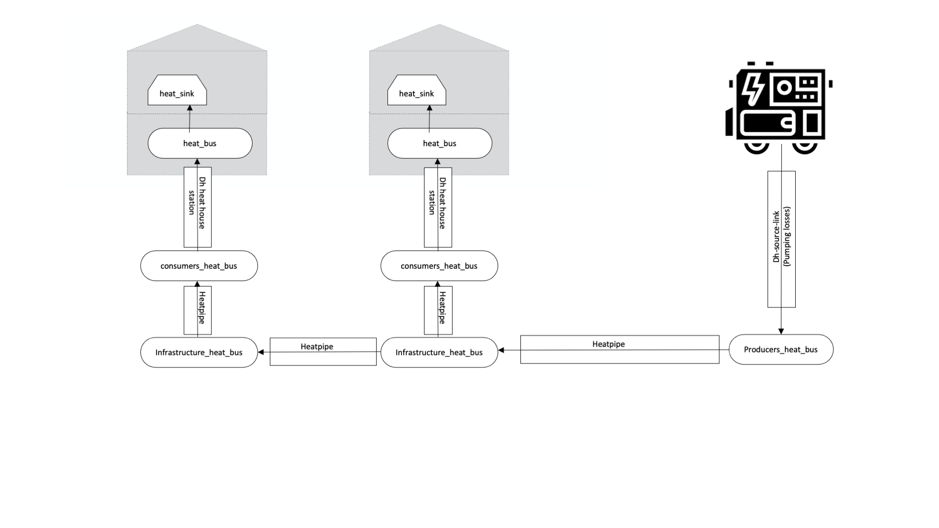
Representation of the district heating network as described above.
Insulation
Thermal insulation represents a possibility to reduce the heat demand of a respective building. For this purpose, an investment decision is used to calculate a U-value and temperature difference dependent saving, which is substracted from the sinks.
Investment
The investment costs help to compare the costs of building new components to the costs of further using existing components instead. The annual savings from building new capacities should compensate the investment costs. The investment method can be applied to any new component to be built. In addition to the usual component parameters, the maximum installable capacity needs to be known. Further, the periodic costs need to be assigned to the investment costs. The periodic costs refer to the defined time horizon. If the time horizon is one year, the periodical costs correspond to the annualized capital costs of an investment.
Non-Convex-Investments
While a linear programming approach is used for normal investment decisions, a mixed integer variable is defined for non-convex investment decisions. The model can thus decide, for example, whether a component should be implemented FULL or NOT. Mixed-integer variables increase the computational effort significantly and should be used with caution.